Differences between revisions 22 and 23
| Deletions are marked like this. | Additions are marked like this. |
| Line 1: | Line 1: |
| #acl All:read |
(Substantially taken from notes made of Ref [1] and [2])
| /FurtherNotes /PowerSpectra |
Contents
Introduction
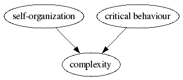
- Combines two interesting phenomena:
Criticality is associated with phase-transitions:
Sub-critical
Critical
Super Critical
Phase I
Boundary
Phase II
Pertubation affects local region
Pertubation can have global effect
Pertubation affects local region
e.g. tapping glass of water
liquid: no change to state
super-cooled: instantaneous phase transition
ice: no change to state
What is needed to form SOC? --> Separation of time-scales
External Driver
Internal Relaxation
Slow
Fast (avalanche)
e.g. build-up of stress in earth's crust (10-10000+ years)
e.g. earthquake (30s-2min)
Threshold Dynamics
(Sornette) An important sub-class of SOC is the out-of-equilibrium systems driven by constant rate, with many interacting components. They possess the following fundamental properties:
- A highly nonlinear behaviour: essentially a threshold response;
- A very slow driving rate;
- A globally stationary regime, characterised by stationary statistical properties;
- Power distributions of event sizes and fractal geometrical propoerties (including long-range correlations).
The threshold dynamics is crucial according to [2] since they accommodate the important separation of time-scales
- Thus, the slipping of the earth's-crust in earth-quake events is a key example of such dynamics.
Example System: Piano
Consider a piano being moved on a carpet floor.
|
Fig. 1 |

- stress builds up in friction between piano and floor
- eventually releases, as piano jumps
- applied force relieved, piano at rest
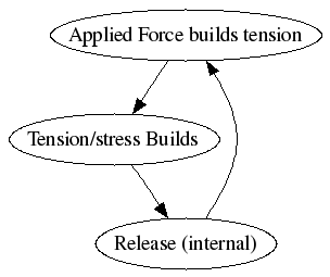
NB: Requires a threshold for release .. consider in the case of the piano, if it were on a plate of ice, applied force would be relieved automatically, quickly. With a threshold for activity (release) tension can build.
Sources of SOC
- Originally believed that only one kind of system was responsible for generating SOC, however, now accepted that various systems can give rise to self-organization to a state without characteristic scale;
- Sources of SOC mentioned in [2] (p.331):
Systems where elements tend to synchronize, but are frustrated by constraints such as open boundary conditions and quenched disorder, leading to a dynamical regime at the edge of synchronization, the SOC state;
So-called extremal models -- SOC is exhibited due to the competition between local strengthening and weaking due to interactions;
SOC also results in systems where the order parameter is tuned in a system exhibiting a critical point, to a vanishingly small, but positive value, ensuring that the corresponding control parameter lies exactly at its critical value for the underlying depinning transition (?);
- Multiplicatively driven systems, such as the spring-block model driven by temporally increasing spring coefficients;
- Conservation laws are also conjectured to be essential for a class of SOC systems -- the scale invariance can sometimes be shown to arise from local conservation laws (e.g. in the sand-pile, sand-grains are conserved except at the boundaries of the pile).
Concepts
Metastable vs. Marginally Stable States
Metastable
system will have many metastable states, since applied force increases strain (e.g. stored elastic energy between piano and floor)
- though stable, therefore, system not at lowest energy state
Marginally Stable
- these states will respond to pertubation either:
- nothing
- small jump (release)
- large jump (release)
hence, there is no scale dependancy, lack any typical time/length scale
- gives rise to algebraic correlation functions (rather than exponential)
Scale Invariance
Refers to a function that retains the same essential form under re-scaling, i.e. a transformation
latex error! exitcode was 2 (signal 0), transscript follows:. For example, the function,
latex error! exitcode was 2 (signal 0), transscript follows:
under re-scaling gives:
latex error! exitcode was 2 (signal 0), transscript follows:
or
latex error! exitcode was 2 (signal 0), transscript follows:
Which is not a simple rescaling of the function f(x). However, consider the function:
latex error! exitcode was 2 (signal 0), transscript follows:
then under re-scaling:
latex error! exitcode was 2 (signal 0), transscript follows:
or
latex error! exitcode was 2 (signal 0), transscript follows:
Consequently, the function is said to not change its character under re-scaling, the system is said to be 'scale-free'. Plotting such a function in log-log space will yield,
latex error! exitcode was 2 (signal 0), transscript follows:
having intercept log(A) and slope
latex error! exitcode was 2 (signal 0), transscript follows:.
Identifying SOC
SOC is identified in a system by at least two properties:
- Power-laws in Spatial correlations or Response distributions;
- Power-laws in (temporal) Power Spectra.
In practice, since it is often easier to obtain Response Distributions rather than the spatial correlation funciton, finding power-laws in the former is often assumed to indicate spatial scale-free behaviour. This is not always the case, but appears a useful (and practical) indicator.
Response Distributions
As mentioned above, often used as a proxy for distrubution of the spatial correlation function. In practice, a vector of response magnitudes to an applied pertubation (at a given system size) is obtained, and a simple histogram is obtained that leads to a probability distribution.
Method: (For a system at a supposed critical state)
- Perturb system at low frequency;
- Measure response of system in terms of energy/reponse-size etc. E.g for sandpile:
Total # grains involved in response (s);
Avalanche lifetimes (time taken for system to become sub-critical) (t).
- Obtain response distributions, and check for algebraic scaling, e.g.
latex error! exitcode was 2 (signal 0), transscript follows:
latex error! exitcode was 2 (signal 0), transscript follows:
Notes
- For positive identification, need to see relationship over a broad (many decade is desirable) region.
Typically, distribution will be bounded by a lower cutoff
latex error! exitcode was 2 (signal 0), transscript follows:
,latex error! exitcode was 2 (signal 0), transscript follows:
corresponding (in this example) to single grain of sand, or movement of single grain in one time step.Further, for finite systems, expect to see a crossover to exponential decay above certain scale. E.g.,
latex error! exitcode was 2 (signal 0), transscript follows:
Further, if "genuine" critical state, crossover scale must be increasing function of system size, i.e.
latex error! exitcode was 2 (signal 0), transscript follows:
, forlatex error! exitcode was 2 (signal 0), transscript follows:
.- Consequences of power-law scaling in response functions:
if
latex error! exitcode was 2 (signal 0), transscript follows:
, average of distribution (e.g.latex error! exitcode was 2 (signal 0), transscript follows:
) will not exist in the limit of the system size;if
latex error! exitcode was 2 (signal 0), transscript follows:
, second moment or "width" of distribution (i.e. standard deviation) will not exist.
Temporal Fluctuations
This asks 'by how much does an event today affect tomorrow, or very far into the future?'. Focus of enquiry is thus on the temporal correlation function:
latex error! exitcode was 2 (signal 0), transscript follows:
where
latex error! exitcode was 2 (signal 0), transscript follows:indicates the average of the variable
latex error! exitcode was 2 (signal 0), transscript follows:at constant
latex error! exitcode was 2 (signal 0), transscript follows:.
Consequently, if there were no correlatin between signal
latex error! exitcode was 2 (signal 0), transscript follows:
and the signallatex error! exitcode was 2 (signal 0), transscript follows:
time units later, then we would expectlatex error! exitcode was 2 (signal 0), transscript follows:
.Now, since
latex error! exitcode was 2 (signal 0), transscript follows:
is related to the power spectrum by cosine transformation we have,latex error! exitcode was 2 (signal 0), transscript follows:
and so,
latex error! exitcode was 2 (signal 0), transscript follows:
Furthermore (see /FurtherNotes), if
latex error! exitcode was 2 (signal 0), transscript follows:
withlatex error! exitcode was 2 (signal 0), transscript follows:
, thenlatex error! exitcode was 2 (signal 0), transscript follows:
will instead of being exponential in decay, has slow logarithmic decay, or in other words, exhibits long-memory effects.For an extended discussion of Power Spectra see /PowerSpectra.
Spatial Correlation Functions
We consider a system described by a field n(r,t) where n represents the local density of particles (for example) in a liquid. 
We have the Correlation Function
latex error! exitcode was 2 (signal 0), transscript follows:
where the spatial coordinates in r are vectors of length d.
Now, for a physical system, away from the critical temperature we might have (say) exponential decay:
latex error! exitcode was 2 (signal 0), transscript follows:
where
latex error! exitcode was 2 (signal 0), transscript follows:
is the correlation length;The correlation length diverges with respect to the absolute distance from the critical temperature:
latex error! exitcode was 2 (signal 0), transscript follows:
However, at the critical point,
latex error! exitcode was 2 (signal 0), transscript follows:
, the correlation function G(r) changes behavior to algebraic dependance:latex error! exitcode was 2 (signal 0), transscript follows:
Divergence of
latex error! exitcode was 2 (signal 0), transscript follows:
is seen to be a signal of lack of characteristic length scale atlatex error! exitcode was 2 (signal 0), transscript follows:
.
Note that the spatial correlation function is for some given time interval. Hence it measures the instantaneous correlation across the dimensions of the system. In practice, it is quite difficult to obtain the spatial correlation function
Extended Numerical Example: The Sandpile
The sandpile system:
- sand grains assumed to drop at either
- random locations
- boundary locations (only)
modelled as a gradient grid: z(i,j) defines slope at position i,j;
that is, z(i,j) = 0 for all positions would indicate a flat pile;
then define
latex error! exitcode was 2 (signal 0), transscript follows:
the threshold/critical slope. If exceeded, assumed that a relaxation event occurs at i,j, propogating (potentially) to neighbourhood of i,j by cellular automata rules:latex error! exitcode was 2 (signal 0), transscript follows:
;latex error! exitcode was 2 (signal 0), transscript follows:
;latex error! exitcode was 2 (signal 0), transscript follows:
;latex error! exitcode was 2 (signal 0), transscript follows:
;latex error! exitcode was 2 (signal 0), transscript follows:
;
i.e. a Moore neighbourhood relaxation
- relaxation algorithm is applied to all super-critical points until none remain, then a further grain is added.
A relationship exists between any of the Abelian sand-pile event-size measurements:
- size (s): total number of topplings in the avalanche;
- area (a): number of distinct sites which toppled;
- life-time (t): duration of the avalanche; and
- radius (r): maximum distance of a toppled site from the origin.
(Sornette) Between any two such measures, a relationship,
latex error! exitcode was 2 (signal 0), transscript follows:
exists, with the exponents being related to one another, e.g.
latex error! exitcode was 2 (signal 0), transscript follows:
For the Abelian sand-pile
latex error! exitcode was 2 (signal 0), transscript follows:in two-dimensions and
latex error! exitcode was 2 (signal 0), transscript follows:.
Implementation
Implemented as: attachment:sand-v070108-1.m
- Initially used gradient approach as above, but instead, moved to a (more realistic?) hieght approach, with gradient found by simple averaging:
   1 function [z0] = gradient(p0,L)
   2
   3 x(:,:,1) = p0(2:L+1,1:L) - p0(2:L+1,2:L+1);
   4 x(:,:,2) = p0(1:L,1:L) - p0(2:L+1,2:L+1);
   5 x(:,:,3) = p0(1:L,2:L+1) - p0(2:L+1,2:L+1);
   6 z = mean(x,3);
   7 z0 = zeros(L+2,L+2);
   8 z0(2:L+1,2:L+1) = -z;
For
- 2D system;
Characteristic size (side-length) L;
- Updating rule:
   1  fall = [2  2  0
   2          2 -6  0
   3          0  0  0];
Yielded avalanch size events (s) as follows:
|
Fig.2 P(s) v. s; boundary-addition only, L = {10,20,30} |

|
|
Fig.3 20x20 Mature sandpile |


Jensen concludes (p.16) that: We conclude that [..] small avalanches in real sandpiles exhibit behavior that is consistent with the expectation of SOC. However, the SOC-like behavior is cut off and overwhelmed by the large avalanches in the system. Hence we must conclude that real physical sandpiles do not exhibit scale-invariant behavior in space and time.
Implementation II
Original BTW set-up:
Only z (gradient) monitored (not pile height);
- Grains added at centre of square;
- Fractal in nature;
|
Fig. Fractal patterns formed with 41x41 scale BTW sand-pile. Colours represent different values of z. |

Critical Response
Linear size l
latex error! exitcode was 2 (signal 0), transscript follows:
that is, the average radius from the pertubation site to the affected lattice points.Total Energy Release s total number of sites that must be relaxed before all sites are under-critical;
Lifetime t total number of simultaneous relaxation procedures that must be performed until all sites are under-critical.
As can be seen in Fig. below, Total Energy Release yielded interesting (and classic) properties for the loglog plot. A region of power-law scaling covering here a decade of scales, then transition at
latex error! exitcode was 2 (signal 0), transscript follows:to an exponential decay process.
|
Fig. Probability distribution for the Total Energy Release (total # sites to be relaxed for sub-critical everywhere) for the fractal sand-pile. Both L=21 and L=41 are shown |

Implementation III
as above, but now with random grain addition (anywhere on 2D grid);
Critical Response
Critical response distributions were prepared by taking a histogram of the vector of response data as mentioned under critical response above. Each showed at least a power-law section of one decade, with switching to exponential decay evident for large event size.
|
|
|
Linear Size |
Total Energy |
Avalanche Lifetime |


Power Spectrum
A Power Spectrum was prepared following the method in [2]:
- Total dissapation counts (# of over-critical sites being relaxed at each time-point) were recorded for each applied pertubation, producing a vector of length avalanche lifetime for each pertubation;
- These vectors were combined by random superposition on an arbitrarily chosen time series (in this case, around an average of 10 points pere time-value was chosen);
- The constructed time-series was then truncated to just the central (major) fluctuations about the mean to take out the start and finish which have only a few vectors added to them;
This series is then used as the time-series t to input to the power-spectrum function [attachment:powspec.m]. Essentially, this applies a DFFT, obtains the normalized magnitude of the response, and takes only half of the symmetric distribution. This is then plotted against f for each F(t), giving the shown distribution.
|
Power-spectrum of the above model |

Discussion
The results presented for the 50x50 model with random grain addition are very similar to that of ref [2]. Here, the same case is analysed for Avalanche Lifetime distributions to yield a power spectrum with exponent -1.57, whilst cluster sizes (Total Energy) gave exponent -1.0. The signature '1/f' case in the paper is that of a 20x20x20 model.
So we would conclude with Jensen that the sand-pile, in its various guieses gives mixed results with respect to SOC. It appears that some systems with some dimensionalities and boundary conditions satisfied can yield the fabled 1/f noise and power-law distributions in spatial/critical response variables. Jensen addresses this point towards the end of his book, when he asks the question of whether 'tuning' is actually required for these so-called 'self-organized' critical systems. It would appear, for the sand-pile at least, that this is true. His main conclusion is that SOC is probably prevalent in the small avalanches of these systems. The larger ones appear to be a more periodic process, and in those systems where SOC fingerprints are not found, are likely over-whelming the SOC dynamics of the small avalanches.
In physical sand-piles, such results are somewhat confirmed, with specific experimental set-ups, such as the rotating drum etc., or using different constituents of the pile (e.g. rice), indicating that as in the computational world, some degree of tuning is required in the physical reality to observe SOC dynamics.
Finite Size Scaling
(Sornette, p.327) In the case of the sand-pile, for measurements from within the set
latex error! exitcode was 2 (signal 0), transscript follows:introduced above we have,
latex error! exitcode was 2 (signal 0), transscript follows:
Where the exponent
latex error! exitcode was 2 (signal 0), transscript follows:determines the variation of the cut-off of the quantity x within the system of system-size L.
However, scaling for the avalanche sizes (s) are in doubt, possibly due to the effect of large avalanches dissipating at the border which strongly influence the statistics.
See Also
Reference
[1] Jensen, H.J., Self-Organized Criticality, Emergent Complex Behavior in Physical and Biological Systems, Cambridge University Press, Cambridge (1998).
[2]
Sornette, D., Critical Phenomena in Natural Sciences, Chaos, Fractals, Sleforganization and Disorder: Concepts and Tools, Springer-Verlag (2000).