Concepts
Alternative names:
- Power spectrum
- Spectral density
- Power spectral density
- Energy spectral density
Method
Implementation: attachment:powspec-v070111-1.m
We want to distinguish the energy contributions of each possible wave-form to the total signal. To do this, we essentially run a Fourier Transform (usually a discrete Fast Fourier Transform (DFFT)), and then simply extract the part of the transform we are after, and present it in an acceptable manner to judge its shape and slope (if any).
|
|
|
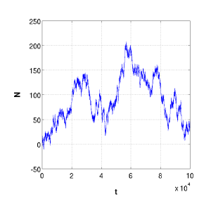
Original signal N(t) |
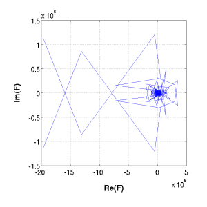
Bare Fourier Transform |
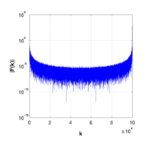
Magnitude Fourier Transform |
Here we have taken the original signal N(t) through the DFFT, and obtained the magnitude of the real and complex components. The DFFT will yield a vector of magnitudes with length n. These can be thought of as the periods of the discrete signals it is searching for. Hence, a response in the third position will be reporting the contribution of waves spanning three numbers in the original signal. It does this by averaging over all possible three unit distances in the data set.
The first value (f(0)) is normally omitted since it is simply the constant-shift term. It is not represented at the other end of the DFFT vector, unlike the other normally symmetric components.
|
|
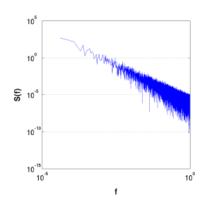
Bare Power Spectrum |
Power spectrum, smoothed |
Since the curve is symmetric in most cases, after omitting the f(0) term, we cut the spectrum in half, and obtain just the LHS. In this case, we have normalised the responses by,
latex error! exitcode was 2 (signal 0), transscript follows:
where conj(F) is the complex conjugate, multiplied element wise by the elements of F, and k is the length of our reduced vector F. Obviously, the numerator has practical significance since it achieves the same job as applying abs(F) to the signal, whilst the denominator is some scaling term.
This procedure gives us our S(f), however, for plotting we will need to convert the periods (just the index numbers) to frequencies:
latex error! exitcode was 2 (signal 0), transscript follows:
for all
latex error! exitcode was 2 (signal 0), transscript follows:. This enables us to plot the Power Spectrum in loglog space as is traditional.
To obtain a clearer presentation of the data, a smoothing operation is performed, taking the moving average of a number of elements, centred at the element of interest.
Common Sequences
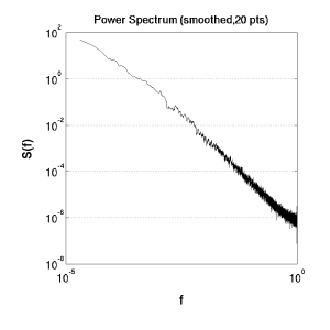
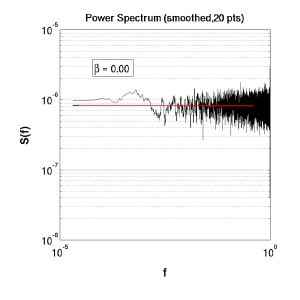
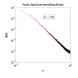
Interest is focussed on the slope of the Power-Spectrum. White (uniform) noise returns a flat S(f) -- the energy being expressed equally across frequencies (see (a) below). Whilst a signal produced via Brownian motion, e.g.
latex error! exitcode was 2 (signal 0), transscript follows:
where e is a random variable in {-1,1}, will give rise to characteristic
latex error! exitcode was 2 (signal 0), transscript follows:slope. Jensen notes that there are many natural processes that give rise to this kind of signal. Indeed, it can also be found by the random superposition of a series of signals generated by a Poisson process.
|
|
(a) White noise |
(b) Brownian noise |
'1/f', 'pink' or 'flicker' noise has a slope of -1, corresponding to 1/f, or
latex error! exitcode was 2 (signal 0), transscript follows:
. As per the article above SciNotes/SelfOrganizedCriticality, this kind of noise is 'special', since apart from falling between the slopes of white and Brownian processes (and so, falling between the white and red noises -- hence, 'pink' noise), a slope of -1 will give rise to the temporal correlation function breaking down from an exponential decay model to one of slow logarithmic decay. In which case, low-frequencies persist indefinitely, and hence the system is said to display 'long-memory' effects. Events that happen today will have slow, building affect on events far into the future -- the system is connected across many time domains.

