Workshop 9 - Generalized linear models
14 September 2011
Basic statistics references
- Logan (2010) - Chpt 16-17
- Quinn & Keough (2002) - Chpt 13-14
Poisson t-test
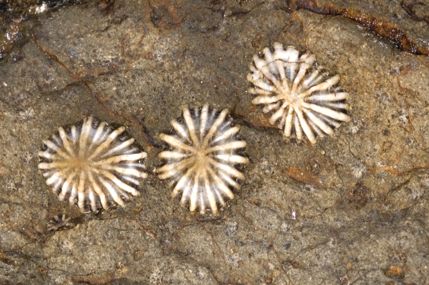
A marine ecologist was interested in examining the effects of wave exposure on the abundance of the striped limpet Siphonaria diemenensis on rocky intertidal shores. To do so, a single quadrat was placed on 10 exposed (to large waves) shores and 10 sheltered shores. From each quadrat, the number of Siphonaria diemenensis were counted.
Download Limpets data set
| Format of limpets.csv data files | |||||||||||||||||||
|---|---|---|---|---|---|---|---|---|---|---|---|---|---|---|---|---|---|---|---|
|
 |
||||||||||||||||||
Open the limpet data set.
The design is clearly a t-test as we are interested in comparing two population means (mean number of striped limpets on exposed and sheltered shores). Recall that a parametric t-test assumes that the residuals (and populations from which the samples are drawn) are normally distributed and equally varied.

- The assumption of normality has been violated?
- The assumption of homogeneity of variance has been violated?
At this point we could transform the data in an attempt to satisfy normality and homogeneity of variance. However, there are likely to be zero values in the data and moreover, it has been demonstrated that transforming count data is not as effective as modelling count data with a Poisson distribution.
- Check the model for lack of fit via:
- Pearson Χ2
Show code
> limpets.resid <- sum(resid(limpets.glm, type = "pearson")^2) > 1 - pchisq(limpets.resid, limpets.glm$df.resid) [1] 0.07874903
#No evidence of a lack of fit - Deviance (G2)
Show code
> 1 - pchisq(limpets.glm$deviance, limpets.glm$df.resid) [1] 0.05286849
#No evidence of a lack of fit - Standardized residuals (plot)
Show code
> plot(limpets.glm) 
- Pearson Χ2
- Estimate the dispersion parameter to evaluate over dispersion in the fitted model
- Via Pearson residuals
Show code
> limpets.resid/limpets.glm$df.resid [1] 1.500731
#No evidence of over dispersion - Via deviance
Show code
> limpets.glm$deviance/limpets.glm$df.resid [1] 1.591496
#No evidence of over dispersion
- Via Pearson residuals
- Compare the expected number of zeros to the actual number of zeros to determine whether the model might be zero inflated.
- Calculate the proportion of zeros in the data
Show code
> limpets.tab <- table(limpets$Count == 0) > limpets.tab/sum(limpets.tab) FALSE TRUE0.85 0.15 - Now work out the proportion of zeros we would expect from a Poisson distribution with a lambda equal to the mean count of limpets in this study.
Show codeClearly there are not more zeros than expected so the data are not zero inflated.
> limpets.mu <- mean(limpets$Count) > cnts <- rpois(1000, limpets.mu) > limpets.tab <- table(cnts == 0) > limpets.tab/sum(limpets.tab) FALSE TRUE0.955 0.045
- Calculate the proportion of zeros in the data
- Wald z-tests (these are equivalent to t-tests)
- Wald Chisq-test. Note that Chisq = z2
- Likelihood ratio test (LRT), analysis of deviance Chisq-tests (these are equivalent to ANOVA)
# OR
# OR
Poisson ANOVA
We once again return to a modified example from Quinn and Keough (2002). In Exercise 1 of Workshop 5, we introduced an experiment by Day and Quinn (1989) that examined how rock surface type affected the recruitment of barnacles to a rocky shore. The experiment had a single factor, surface type, with 4 treatments or levels: algal species 1 (ALG1), algal species 2 (ALG2), naturally bare surfaces (NB) and artificially scraped bare surfaces (S). There were 5 replicate plots for each surface type and the response (dependent) variable was the number of newly recruited barnacles on each plot after 4 weeks.
Download Day data set
| Format of day.csv data files | |||||||||||||||||||||||
|---|---|---|---|---|---|---|---|---|---|---|---|---|---|---|---|---|---|---|---|---|---|---|---|
|
 |
||||||||||||||||||||||
We previously analysed these data with via a classic linear model (ANOVA) as the data appeared to conform to the linear model assumptions. Alternatively, we could analyse these data with a generalized linear model (Poisson error distribution). Note that as the boxplots were all fairly symmetrical and equally varied, and the sample means are well away from zero (in fact there are no zero's in the data) we might suspect that whether we fit the model as a linear or generalized linear model is probably not going to be of great consequence. Nevertheless, it does then provide a good comparison between the two frameworks.

- Check the model for lack of fit via:
- Pearson Χ2
Show code
> day.resid <- sum(resid(day.glm, type = "pearson")^2) > 1 - pchisq(day.resid, day.glm$df.resid) [1] 0.3641093
#No evidence of a lack of fit - Standardized residuals (plot)
Show code
> plot(day.glm) 
- Pearson Χ2
- Estimate the dispersion parameter to evaluate over dispersion in the fitted model
- Via Pearson residuals
Show code
> day.resid/day.glm$df.resid [1] 1.083574
#No evidence of over dispersion - Via deviance
Show code
> day.glm$deviance/day.glm$df.resid [1] 1.075851
#No evidence of over dispersion
- Via Pearson residuals
- Compare the expected number of zeros to the actual number of zeros to determine whether the model might be zero inflated.
- Calculate the proportion of zeros in the data
Show code
> day.tab <- table(day$Count == 0) > day.tab/sum(day.tab) numeric(0) - Now work out the proportion of zeros we would expect from a Poisson distribution with a lambda equal to the mean count of day in this study.
Show codeClearly there are not more zeros than expected so the data are not zero inflated.
> day.mu <- mean(day$Count) > cnts <- rpois(1000, day.mu) > day.tab <- table(cnts == 0) > day.tab/sum(day.tab) numeric(0)
- Calculate the proportion of zeros in the data
- Wald z-tests (these are equivalent to t-tests)
- Wald Chisq-test.
- Likelihood ratio test (LRT), analysis of deviance Chisq-tests (these are equivalent to ANOVA)
# OR
# OR
- Cell (population) means
Show code#On a link (log) scaleOr the long way
> day.means <- predict(day.glm, newdata = data.frame(TREAT = levels(day$TREAT)), > se = T) > day.means <- data.frame(day.means[1], day.means[2]) > rownames(day.means) <- levels(day$TREAT) > day.ci <- qt(0.975, day.glm$df.residual) * day.means[, 2] > day.means <- data.frame(day.means, lwr = day.means[, 1] - day.ci, > upr = day.means[, 1] + day.ci) fit se.fit lwr uprALG1 3.109061 0.09449112 2.908749 3.309373ALG2 3.346389 0.08391814 3.168491 3.524288NB 2.708050 0.11547003 2.463265 2.952836S 2.580217 0.12309146 2.319275 2.841159
#On the scale of the response> day.means <- predict(day.glm, newdata = data.frame(TREAT = levels(day$TREAT)), > se = T, type = "response") > day.means <- data.frame(day.means[1], day.means[2]) > rownames(day.means) <- levels(day$TREAT) > day.ci <- qt(0.975, day.glm$df.residual) * day.means[, 2] > day.means <- data.frame(day.means, lwr = day.means[, 1] - day.ci, > upr = day.means[, 1] + day.ci) fit se.fit lwr uprALG1 22.4 2.116601 17.913006 26.88699ALG2 28.4 2.383275 23.347683 33.45232NB 15.0 1.732051 11.328217 18.67178S 13.2 1.624807 9.755563 16.64444Show code#On a link (log) scale> cmat <- cbind(c(1, 0, 0, 0), c(1, 1, 0, 0), c(1, 0, 1, 0), c(1, > 0, 0, 1)) > day.mu <- t(day.glm$coef %*% cmat) > day.se <- sqrt(diag(t(cmat) %*% vcov(day.glm) %*% cmat)) > day.means <- data.frame(fit = day.mu, se = day.se) > rownames(day.means) <- levels(day$TREAT) > day.ci <- qt(0.975, day.glm$df.residual) * day.se > day.means <- data.frame(day.means, lwr = day.mu - day.ci, upr = day.mu + > day.ci) fit se lwr uprALG1 3.109061 0.09449112 2.908749 3.309373ALG2 3.346389 0.08391814 3.168491 3.524288NB 2.708050 0.11547003 2.463265 2.952836S 2.580217 0.12309146 2.319275 2.841159
#On a response scale> cmat <- cbind(c(1, 0, 0, 0), c(1, 1, 0, 0), c(1, 0, 1, 0), c(1, > 0, 0, 1)) > day.mu <- t(day.glm$coef %*% cmat) > day.se <- sqrt(diag(t(cmat) %*% vcov(day.glm) %*% cmat)) * abs(poisson()$mu.eta(day.mu)) > day.mu <- exp(day.mu) > day.se <- sqrt(diag(vcov(day.glm) %*% cmat)) * day.mu > day.means <- data.frame(fit = day.mu, se = day.se) > rownames(day.means) <- levels(day$TREAT) > day.ci <- qt(0.975, day.glm$df.residual) * day.se > day.means <- data.frame(day.means, lwr = day.mu - day.ci, upr = day.mu + > day.ci) fit se lwr uprALG1 22.4 2.116601 17.913006 26.88699ALG2 28.4 2.383275 23.347683 33.45232NB 15.0 1.732051 11.328217 18.67178S 13.2 1.624807 9.755563 16.64444 - Differences between each treatment mean and the global mean
Show code#On a link (log) scale
> cmat <- rbind(c(1, 0, 0, 0), c(1, 1, 0, 0), c(1, 0, 1, 0), c(1, > 0, 0, 1)) > gm.cmat <- apply(cmat, 2, mean) > for (i in 1:nrow(cmat)) { > cmat[i, ] <- cmat[i, ] - gm.cmat > } > day.glm$coef %*% gm.cmat > day.mu <- t(day.glm$coef %*% t(cmat)) > day.se <- sqrt(diag(cmat %*% vcov(day.glm) %*% t(cmat))) > day.means <- data.frame(fit = day.mu, se = day.se) > rownames(day.means) <- levels(day$TREAT) > day.ci <- qt(0.975, day.glm$df.residual) * day.se > day.means <- data.frame(day.means, lwr = day.mu - day.ci, upr = day.mu + > day.ci) fit se lwr uprALG1 0.1731317 0.08510443 -0.007281663 0.3535450ALG2 0.4104599 0.07937005 0.242202862 0.5787169NB -0.2278791 0.09718613 -0.433904466 -0.0218537S -0.3557125 0.10175575 -0.571425004 -0.1399999
#On a response scale> cmat <- rbind(c(1, 0, 0, 0), c(1, 1, 0, 0), c(1, 0, 1, 0), c(1, > 0, 0, 1)) > gm.cmat <- apply(cmat, 2, mean) > for (i in 1:nrow(cmat)) { > cmat[i, ] <- cmat[i, ] - gm.cmat > } > day.glm$coef %*% gm.cmat > day.mu <- t(day.glm$coef %*% t(cmat)) > day.se <- sqrt(diag(cmat %*% vcov(day.glm) %*% t(cmat))) * abs(poisson()$mu.eta(day.mu)) > day.mu <- exp(abs(day.mu)) > day.means <- data.frame(fit = day.mu, se = day.se) > rownames(day.means) <- levels(day$TREAT) > day.ci <- qt(0.975, day.glm$df.residual) * day.se > day.means <- data.frame(day.means, lwr = day.mu - day.ci, upr = day.mu + > day.ci) fit se lwr uprALG1 1.189023 0.10119110 0.9745071 1.403538ALG2 1.507511 0.11965122 1.2538616 1.761160NB 1.255933 0.07738159 1.0918918 1.419975S 1.427197 0.07129761 1.2760529 1.578341
Poisson t-test with overdispersion
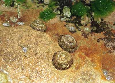
The same marine ecologist that featured earlier was also interested in examining the effects of wave exposure on the abundance of another intertidal marine limpet Cellana tramoserica on rocky intertidal shores. Again, a single quadrat was placed on 10 exposed (to large waves) shores and 10 sheltered shores. From each quadrat, the number of smooth limpets (Cellana tramoserica) were counted.
Download LimpetsSmooth data set
| Format of limpetsSmooth.csv data files | |||||||||||||||||||
|---|---|---|---|---|---|---|---|---|---|---|---|---|---|---|---|---|---|---|---|
|
 |
||||||||||||||||||
Open the limpetsSmooth data set.
- Check the model for lack of fit via:
- Pearson Χ2
Show code
> limpets.resid <- sum(resid(limpets.glm, type = "pearson")^2) > 1 - pchisq(limpets.resid, limpets.glm$df.resid) [1] 4.440892e-16
#No evidence of a lack of fit - Deviance (G2)
Show code
> 1 - pchisq(limpets.glm$deviance, limpets.glm$df.resid) [1] 1.887379e-15
#No evidence of a lack of fit - Standardized residuals (plot)
Show code
> plot(limpets.glm) 
- Pearson Χ2
- Estimate the dispersion parameter to evaluate over dispersion in the fitted model
- Via Pearson residuals
Show code
> limpets.resid/limpets.glm$df.resid [1] 6.358197
#Evidence of over dispersion - Via deviance
Show code
> limpets.glm$deviance/limpets.glm$df.resid [1] 6.177846
#Evidence of over dispersion
- Via Pearson residuals
- Compare the expected number of zeros to the actual number of zeros to determine whether the model might be zero inflated.
- Calculate the proportion of zeros in the data
Show code
> limpets.tab <- table(limpets$Count == 0) > limpets.tab/sum(limpets.tab) FALSE TRUE0.9 0.1 - Now work out the proportion of zeros we would expect from a Poisson distribution with a lambda equal to the mean count of limpets in this study.
Show codeClearly there are not more zeros than expected so the data are not zero inflated.
> limpets.mu <- mean(limpets$Count) > cnts <- rpois(1000, limpets.mu) > limpets.tab <- table(cnts == 0) > limpets.tab/sum(limpets.tab) FALSE TRUE0.999 0.001
- Calculate the proportion of zeros in the data
Clearly there is an issue of with overdispersion. There are multiple potential reasons for this. It could be that there are major sources of variability that are not captured within the sampling design. Alternatively it could be that the data are very clumped. For example, often species abundances are clumped - individuals are either not present, or else when they are present they occur in groups.
- Explore the distribution of counts from each population
Show code
> boxplot(Count ~ Shore, data = limpets) > rug(jitter(limpets$Count), side = 2) 
- Fit the model with a quasipoisson distribution in which the dispersion factor (lambda) is not assumed to be 1.
The degree of variability (and how this differs from the mean) is estimated and the dispersion factor is incorporated.
Show code
> limpets.glmQ <- glm(Count ~ Shore, family = quasipoisson, data = limpets) - t-tests
- Wald F-test. Note that F = t2
Show code> summary(limpets.glmQ) Call:glm(formula = Count ~ Shore, family = quasipoisson, data = limpets)Deviance Residuals:Min 1Q Median 3Q Max-3.6352 -2.6303 -0.4752 1.0449 5.3451Coefficients:Estimate Std. Error t value Pr(>|t|)(Intercept) 2.2925 0.2534 9.046 4.08e-08 ***Shoresheltered -0.9316 0.4767 -1.954 0.0664 .---Signif. codes: 0 ‘***’ 0.001 ‘**’ 0.01 ‘*’ 0.05 ‘.’ 0.1 ‘ ’ 1(Dispersion parameter for quasipoisson family taken to be 6.358223)Null deviance: 138.18 on 19 degrees of freedomResidual deviance: 111.20 on 18 degrees of freedomAIC: NANumber of Fisher Scoring iterations: 5Show code> library(car) > Anova(limpets.glmQ, test.statistic = "F") Analysis of Deviance Table (Type II tests)Response: CountSS Df F Pr(>F)Shore 26.978 1 4.243 0.05417 .Residuals 114.448 18---Signif. codes: 0 ‘***’ 0.001 ‘**’ 0.01 ‘*’ 0.05 ‘.’ 0.1 ‘ ’ 1
#OR> anova(limpets.glmQ, test = "F") Analysis of Deviance TableModel: quasipoisson, link: logResponse: CountTerms added sequentially (first to last)Df Deviance Resid. Df Resid. Dev F Pr(>F)NULL 19 138.18Shore 1 26.978 18 111.20 4.243 0.05417 .---Signif. codes: 0 ‘***’ 0.001 ‘**’ 0.01 ‘*’ 0.05 ‘.’ 0.1 ‘ ’ 1 - Fit the model with a negative binomial distribution (which accounts for the clumping).
Show codeCheck the fit
> limpets.glmNB <- glm.nb(Count ~ Shore, data = limpets) Show code> limpets.resid <- sum(resid(limpets.glmNB, type = "pearson")^2) > 1 - pchisq(limpets.resid, limpets.glmNB$df.resid) [1] 0.4333663#Deviance> 1 - pchisq(limpets.glmNB$deviance, limpets.glmNB$df.resid) [1] 0.215451- Wald z-tests (these are equivalent to t-tests)
- Wald Chisq-test. Note that Chisq = z2
Show code> summary(limpets.glmNB) Call:glm.nb(formula = Count ~ Shore, data = limpets, init.theta = 1.283382111,link = log)Deviance Residuals:Min 1Q Median 3Q Max-1.8929 -1.0926 -0.2313 0.3943 1.5320Coefficients:Estimate Std. Error z value Pr(>|z|)(Intercept) 2.2925 0.2967 7.727 1.1e-14 ***Shoresheltered -0.9316 0.4377 -2.128 0.0333 *---Signif. codes: 0 ‘***’ 0.001 ‘**’ 0.01 ‘*’ 0.05 ‘.’ 0.1 ‘ ’ 1(Dispersion parameter for Negative Binomial(1.2834) family taken to be 1)Null deviance: 26.843 on 19 degrees of freedomResidual deviance: 22.382 on 18 degrees of freedomAIC: 122.02Number of Fisher Scoring iterations: 1Theta: 1.283Std. Err.: 0.5062 x log-likelihood: -116.018Show code> library(car) > Anova(limpets.glmNB, test.statistic = "Wald") Analysis of Deviance Table (Type II tests)Response: CountDf Chisq Pr(>Chisq)Shore 1 4.5297 0.03331 *Residuals 18---Signif. codes: 0 ‘***’ 0.001 ‘**’ 0.01 ‘*’ 0.05 ‘.’ 0.1 ‘ ’ 1Analysis of Deviance TableModel: Negative Binomial(1.2834), link: logResponse: CountTerms added sequentially (first to last)Df Deviance Resid. Df Resid. Dev F Pr(>F)NULL 19 26.843Shore 1 4.4611 18 22.382 4.4611 0.03468 *---Signif. codes: 0 ‘***’ 0.001 ‘**’ 0.01 ‘*’ 0.05 ‘.’ 0.1 ‘ ’ 1Analysis of Deviance TableModel: Negative Binomial(1.2834), link: logResponse: CountTerms added sequentially (first to last)Df Deviance Resid. Df Resid. Dev P(>|Chi|)NULL 19 26.843Shore 1 4.4611 18 22.382 0.03468 *---Signif. codes: 0 ‘***’ 0.001 ‘**’ 0.01 ‘*’ 0.05 ‘.’ 0.1 ‘ ’ 1
Poisson t-test with zero-inflation
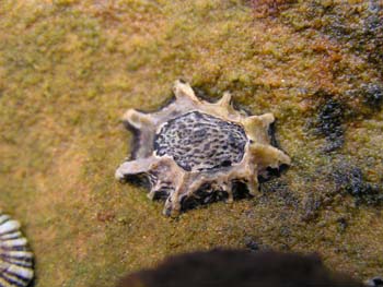
Yet again our rather fixated marine ecologist has returned to the rocky shore with an interest in examining the effects of wave exposure on the abundance of yet another intertidal marine limpet Patelloida latistrigata on rocky intertidal shores. It would appear that either this ecologist is lazy, is satisfied with the methodology or else suffers from some superstition disorder (that prevents them from deviating too far from a series of tasks), and thus, yet again, a single quadrat was placed on 10 exposed (to large waves) shores and 10 sheltered shores. From each quadrat, the number of scaley limpets (Patelloida latistrigata) were counted. Initially, faculty were mildly interested in the research of this ecologist (although lets be honest, most academics usually only display interest in the work of the other members of their school out of politeness - Oh I did not say that did I?). Nevertheless, after years of attending seminars by this ecologist in which the only difference is the target species, faculty have started to display more disturbing levels of animosity towards our ecologist. In fact, only last week, the members of the school's internal ARC review panel (when presented with yet another wave exposure proposal) were rumored to take great pleasure in concocting up numerous bogus applications involving hedgehogs and balloons just so they could rank our ecologist proposal outside of the top 50 prospects and ... Actually, I may just have digressed!
Download LimpetsScaley data set
| Format of limpetsScaley.csv data files | |||||||||||||||||||
|---|---|---|---|---|---|---|---|---|---|---|---|---|---|---|---|---|---|---|---|
|
 |
||||||||||||||||||
Open the limpetsSmooth data set.
- Explore the distribution of counts from each population
Show code
> boxplot(Count ~ Shore, data = limpets) > rug(jitter(limpets$Count), side = 2) 
- Compare the expected number of zeros to the actual number of zeros to determine whether the model might be zero inflated.
- Calculate the proportion of zeros in the data
Show code
> limpets.tab <- table(limpets$Count == 0) > limpets.tab/sum(limpets.tab) FALSE TRUE0.75 0.25 - Now work out the proportion of zeros we would expect from a Poisson distribution with a lambda equal to the mean count of limpets in this study.
Show codeClearly there are not more zeros than expected so the data are not zero inflated.
> limpets.mu <- mean(limpets$Count) > cnts <- rpois(1000, limpets.mu) > limpets.tab <- table(cnts == 0) > limpets.tab/sum(limpets.tab) FALSE TRUE0.91 0.09
- Calculate the proportion of zeros in the data
pscl vcd colorspace grid gam coda lattice multcomp mvtnorm gmodels car survival splines nnet MASS R2HTML stats graphics grDevices utils datasets methods base
- Check the model for lack of fit via:
- Pearson Χ2
Show code
> limpets.resid <- sum(resid(limpets.zip, type = "pearson")^2) > 1 - pchisq(limpets.resid, limpets.zip$df.resid) [1] 0.2810221
#No evidence of a lack of fit
- Pearson Χ2
- Estimate the dispersion parameter to evaluate over dispersion in the fitted model
- Via Pearson residuals
Show code
> limpets.resid/limpets.zip$df.resid [1] 1.168722
#No evidence of over dispersion
- Via Pearson residuals
- Wald z-tests (these are equivalent to t-tests)
- Chisq-test. Note that Chisq = z2
- F-test. Note that Chisq = z2