Workshop 8 - Frequency analysis and generalized linear models

29 August 2011

Topics

Chi-square tests
- Exercise 1
Contingency analysis
Log-linear models
- Exercise 5
- Exercise 6

Basic statistics references

Logan (2010) - Chpt 16-17
Quinn & Keough (2002) - Chpt 13-14

Analysis of frequencies.

Goodness of fit test

A fictitious plant ecologist sampled 90 shrubs of a dioecious plant in a forest, and each plant was classified as being either male or female. The ecologist was interested in the sex ratio and whether it differed from 50:50. The observed counts and the predicted (expected) counts based on a theoretical 50:50 sex ratio follow.

Format of fictitious plant sex ratios - note, not a file

Expected and Observed data (50:50 sex ratio).

	Female	Male	Total
Observed	40	50	90
Expected	45	45	90

Note, it is not necessary to open or create a data file for this question.

Q1-1. First, what is the appropriate test

to examine the sex ratio of these plants?

Q1-2. What null hypothesis is being tested by this test?

Q1-3. What are the degrees of freedom are associated with this data for this test?

Q1-4. Perform a Goodness-of-fit test

to test the null hypothesis that these data came from a population with a 50:50 sex ratio (hint). Identify the following:

Show code

> chisq.test(c(40, 50))

Chi-squared test for given probabilities

data: c(40, 50)

X-squared = 1.1111, df = 1, p-value = 0.2918

X² statistic
df
P value

Q1-5. What are your conclusions (statistical and biological)?

Lets now extend this fictitious endeavor. Recent studies on a related species of shrub have suggested a 30:70 female:male sex ratio. Knowing that our plant ecologist had similar research interests, the authors contacted her to inquire whether her data contradicted their findings.

Q1-6. Using the same observed data, test the null hypothesis

that these data came from a population with a 30:70 sex ratio (hint). From a 30:70 female:male sex ratio, what are the expected frequency counts of females and males from 90 individuals and what is the X² statistic?.

Show code

> chisq.test(c(40, 50), p = c(0.3, 0.7))

Chi-squared test for given probabilities

data: c(40, 50)

X-squared = 8.9418, df = 1, p-value = 0.002787

> chisq.test(c(40, 50), p = c(0.3, 0.7))$exp

[1] 27 63

Expected number of females
Expected number of males
X² statistic

Q1-7. Do the plant ecologist's data dispute the findings of the other studies? (y or n)

Contingency tables

Here is a modified example from Quinn and Keough (2002). Following fire, French and Westoby (1996) cross-classified plant species by two variables: whether they regenerated by seed only or vegetatively and whether they were dispersed by ant or vertebrate vector. The two variables could not be distinguished as response or predictor since regeneration mechanisms could just as conceivably affect dispersal mode as vice versa.

Download French data set

Format of french.csv data files

REGEN	DISP	COUNT
seed	ant	25
seed	vert	6
veg	ant	36
veg	vert	21

REGEN	Categorical listing of the plants regeneration mode.
DISP	Categorical listing of the plants dispersal mode.
COUNT	The observed number of individuals in each category.

	DISPERSAL MODE
REGENERATION MODE	ANT	Vertebrate
SeedOnly	25	6
Vegetative	61	21

Open the french data file. HINT.

Show code

> french <- read.table("french.csv", header = T, sep = ",", strip.white = T)

> head(french)

regen disp count

1 seed ant 25

2 seed vert 6

3 veg ant 36

4 veg vert 21

Q2-1. What null hypothesis is being tested by this test?

Q2-2. Generate a cross table

out of the dataset in preparation for frequency analysis (HINT).

Show code

> french.tab <- xtabs(count ~ regen + disp, data = french)

> french.tab

disp

regen ant vert

seed 25 6

veg 36 21

Q2-3. Fit

a 2 x 2 (two way) contingency table

(HINT), and explore the main assumption of the test by examining the expected frequencies (HINT).

Show code

> french.x2 <- chisq.test(french.tab, correct = F)

> french.x2$exp

disp

regen ant vert

seed 21.48864 9.511364

veg 39.51136 17.488636

Q2-4. If the assumption is OK, test this null hypothesis and identify the following.

Show code

> french.x2

Pearson's Chi-squared test

data: french.tab

X-squared = 2.8872, df = 1, p-value = 0.08929

X² statistic
df
P value

Q2-5. What are your conclusions (statistical and biological)?

Contingency tables

Arrington et al. (2002) examined the frequency with which African, Neotropical and North American fishes have empty stomachs and found that the mean percentage of empty stomachs was around 16.2%. As part of the investigation they were interested in whether the frequency of empty stomachs was related to dietary items. The data were separated into four major trophic classifications (detritivores, omnivores, invertivores, and piscivores) and whether the fish species had greater or less than 16.2% of individuals with empty stomachs. The number of fish species in each category combination was calculated and a subset of that (just the diurnal fish) is provided.

Download Arrington data set

Format of arrington.csv data file

STOMACH	TROPHIC
< 16.2	DET
..	..
< 16.2	OMN
..	..
< 16.2	PISC
..	..
< 16.2	INV
..	..

STOMACH	Categorical listing of the proportion of individuals in the species with empty stomachs (< 16.2% or > 16.2%).
TROPHIC	Categorical listing of the trophic classification (DET = detritovore, OMN = omnivore, INV = invertivore, PISC = piscivore).

	% Stomachs empty
Trophic classification	< 16.2	> 16.2
DET	18	4
OMN	45	8
INV	58	15
PISC	16	34

Open the arrington data file (HINT).

Show code

> arrington <- read.table("arrington.csv", header = T, sep = ",",

> strip.white = T)

> head(arrington)

STOMACH TROPHIC

1 <16.2 DET

2 <16.2 DET

3 <16.2 DET

4 <16.2 DET

5 <16.2 DET

6 <16.2 DET

Note the format of the data file. Rather than including a compilation of the observed counts, this data file lists the categories for each individual. This example will demonstrate how to analyse two-way contingency tables from such data files. Each row of the data set represents a separate species of fish that is then cross categorised according to whether the proportion of individuals of that species with empty stomachs was higher or lower than the overall average (16.2%) and to what trophic group they belonged.

Q3-1. Generate a cross table

out of the raw data file in preparation for the contingency table (HINT).

Show code

> arrington.tab <- table(arrington)

> arrington.tab

TROPHIC

STOMACH DET INV OMN PISC

<16.2 18 58 45 16

>16.2 4 15 8 34

Q3-2. Fit the model (HINT), test the assumptions (HINT) and, using a two-way contingency table,

test the null hypothesis that the percentage of empty stomachs was independent of trophic classification (HINT). What would you conclude form the analysis?

Show code

> arrington.x2 <- chisq.test(arrington.tab)

> arrington.x2$exp

TROPHIC

STOMACH DET INV OMN PISC

<16.2 15.222222 50.5101 36.67172 34.59596

>16.2 6.777778 22.4899 16.32828 15.40404

> arrington.x2

Pearson's Chi-squared test

data: arrington.tab

X-squared = 43.8346, df = 3, p-value = 1.636e-09

Write the results out as though you were writing a research paper/thesis. For example (select the phrase that applies and fill in gaps with your results):
The percentage of empty stomachs was (choose the correct option)
trophic classification. (X² = , df = , P = ).

Q3-3. Generate the residuals (HINT) associated with the above contingency test and complete the following table of standardized residuals.

Show code

> arrington.x2$res

TROPHIC

STOMACH DET INV OMN PISC

<16.2 0.7119647 1.0538695 1.3752759 -3.1615926

>16.2 -1.0669740 -1.5793639 -2.0610342 4.7380678

	< 16.2%	> 16.2%
DET
OMN
INV
PISC

Q3-4. What further conclusions would you draw from the standardized residuals?

Contingency tables

Here is an example (13.5) from Fowler, Cohen and Parvis (1998). A field biologist collected leaf litter from a 1 m² quadrats randomly located on the ground at night in two locations - one was on clay soil the other on chalk soil. The number of woodlice of two different species (Oniscus and Armadilidium) were collected and it is assumed that all woodlice undertake their nocturnal activities independently. The number of woodlice are in the following contingency table.

Download Woodlice data set

Format of Woodlice data set

	WOODLICE SPECIES
SOIL TYPE	Oniscus	Armadilidium
Clay	14	6
Chalk	22	46

Open the woodlice data file. HINT.

Show code

> woodlice <- read.table("woodlice.csv", header = T, sep = ",",

> strip.white = T)

> head(woodlice)

SOIL SPECIES COUNTS

1 Clay oniscus 14

2 Clay armadilidium 6

3 Chalk oniscus 22

4 Chalk armadilidium 46

Q4-1. What null hypothesis is being tested by this test?

Q4-2. Generate a cross table

out of the dataset in preparation for frequency analysis (HINT).

Show code

> woodlice.tab <- xtabs(COUNTS ~ SOIL + SPECIES, data = woodlice)

> woodlice.tab

SPECIES

SOIL armadilidium oniscus

Chalk 46 22

Clay 6 14

Q4-3. Fit

a 2 x 2 (two way) contingency table

(HINT), and explore the main assumption of the test by examining the expected frequencies (HINT).

Show code

> woodlice.x2 <- chisq.test(woodlice.tab, correct = F)

> woodlice.x2$exp

SPECIES

SOIL armadilidium oniscus

Chalk 40.18182 27.818182

Clay 11.81818 8.181818

Q4-4. If the assumption is OK, test this null hypothesis (HINT) and identify the following.

Show code

> woodlice.x2

Pearson's Chi-squared test

data: woodlice.tab

X-squared = 9.061, df = 1, p-value = 0.002611

X² statistic
df
P value

Q4-5. Generate the residuals (HINT) associated with the above contingency test and complete the following table of standardized residuals.

	oniscus	armadilidium
CLAY
CHALK

Q4-6. What are your conclusions (statistical and biological)?

Logistic regression

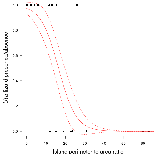
Polis et al. (1998) were intested in modelling the presence/absence of lizards (Uta sp.) against the perimeter to area ratio of 19 islands in the Gulf of California.

Download Polis data set

Format of polis.csv data file

ISLAND	RATIO	PA
Bota	15.41	1
Cabeza	5.63	1
Cerraja	25.92	1
Coronadito	15.17	0
..	..	..

ISLAND	Categorical listing of the name of the 19 islands used - variable not used in analysis.
RATIO	Ratio of perimeter to area of the island.
PA	Presence (1) or absence (0) of Uta lizards on island.

Open the polis data file (HINT).

Show code

> polis <- read.table("polis.csv", header = T, sep = ",", strip.white = T)

> head(polis)

ISLAND RATIO PA

1 Bota 15.41 1

2 Cabeza 5.63 1

3 Cerraja 25.92 1

4 Coronadito 15.17 0

5 Flecha 13.04 1

6 Gemelose 18.85 0

Q5-1. What is the null hypothesis of interest?

Q5-2. Fitting the general linear model with a binomial error distribution (logit linkage)

(HINT).

Show code

> polis.glm <- glm(PA ~ RATIO, family = binomial, data = polis)

Check the model for lack of fit via:
- Pearson Χ²
  Show code
  
  [1] 0.5715331
  
  #No evidence of a lack of fit
- Deviance (G²)
  Show code
  
  [1] 0.6514215
  
  #No evidence of a lack of fit
Estimate the dispersion parameter to evaluate over dispersion in the fitted model
- Via Pearson residuals
  Show code
  
  [1] 0.9019219
  
  #No evidence of over dispersion
- Via deviance
  Show code
  
  [1] 0.8365126
  
  #No evidence of over dispersion
Compare the expected number of zeros to the actual number of zeros to determine whether the model might be zero inflated.
- Calculate the proportion of zeros in the data
  Show code
  
  FALSE TRUE
  0.5263158 0.4736842
- Assuming a probability of 0.5 for each trial, you would expect roughly 50:50 (50%) zeros and ones. So the data are not zero inflated.

Q5-3. As the diagnostics do not indicate any issues with the data or the fitted model, identify and interpret the following (HINT);

Show code

> polis.glm <- glm(PA ~ RATIO, family = binomial, data = polis)

> summary(polis.glm)

Call:

glm(formula = PA ~ RATIO, family = binomial, data = polis)

Deviance Residuals:

Min 1Q Median 3Q Max

-1.6067 -0.6382 0.2368 0.4332 2.0986

Coefficients:

Estimate Std. Error z value Pr(>|z|)

(Intercept) 3.6061 1.6953 2.127 0.0334 *

RATIO -0.2196 0.1005 -2.184 0.0289 *

---

Signif. codes: 0 ‘***’ 0.001 ‘**’ 0.01 ‘*’ 0.05 ‘.’ 0.1 ‘ ’ 1

(Dispersion parameter for binomial family taken to be 1)

Null deviance: 26.287 on 18 degrees of freedom

Residual deviance: 14.221 on 17 degrees of freedom

AIC: 18.221

Number of Fisher Scoring iterations: 6

sample constant (β₀)
sample slope (β₁)
Wald statistic (z value) for main H₀
P-value for main H₀
r² value (HINT)
Show code

[1] 0.4590197

Q5-3.Another way ot test the fit of the model, and thus test the H₀ that β₁ = 0, is to compare the fit of the full model to the reduce model via ANOVA. Perform this ANOVA (HINT) and identify the following

Show code

> anova(polis.glm, test = "Chisq")

Analysis of Deviance Table

Model: binomial, link: logit

Response: PA

Terms added sequentially (first to last)

Df Deviance Resid. Df Resid. Dev P(>|Chi|)

NULL 18 26.287

RATIO 1 12.066 17 14.221 0.0005134 ***

---

Signif. codes: 0 ‘***’ 0.001 ‘**’ 0.01 ‘*’ 0.05 ‘.’ 0.1 ‘ ’ 1

G² statistic
df
P value

Q5-4. Construct a scatterplot of the presence/absence of Uta lizards against perimeter to area ratio for the 19 islands (HINT). Add to this plot, the predicted probability of occurances from the logistic regression (as well as 66% confidence interval - standard error). (HINT)

Show code

> par(mar = c(4, 5, 0, 0))

> plot(PA ~ RATIO, data = polis, type = "n", ann = F, axes = F)

> points(PA ~ RATIO, data = polis, pch = 16)

> xs <- seq(0, 70, l = 1000)

> ys <- predict(polis.glm, newdata = data.frame(RATIO = xs), type = "response",

> se = T)

> points(ys$fit ~ xs, col = "red", type = "l")

> lines(ys$fit - 1 * ys$se.fit ~ xs, col = "red", type = "l", lty = 2)

> lines(ys$fit + 1 * ys$se.fit ~ xs, col = "red", type = "l", lty = 2)

> axis(1)

> mtext("Island perimeter to area ratio", 1, cex = 1.5, line = 3)

> axis(2, las = 2)

> mtext(expression(paste(italic(Uta), " lizard presence/absence")),

> 2, cex = 1.5, line = 3)

> box(bty = "l")

Q5-5. Calculate the LD50 (in this case, the perimeter to area ratio with a predicted probability of 0.5) from the fitted model (HINT).

Show code

> -polis.glm$coef[1]/polis.glm$coef[2]

(Intercept)

16.4242

Islands above this ratio are not predicted to contain lizards and islands above this ratio are expected to have lizards.

Q5-6. Examine the odds ratio for the occurrence of Uta lizards.

Show code

> library(biology)

> odds.ratio(polis.glm)

Odds ratio Lower 95% CI Upper 95% CI

RATIO 0.8028734 0.659303 0.9777077

Q5-7. What are your conclusions (statistical and biological)?

Log-linear modelling

Roberts (1993) was intested in examining the interaction between the presence of dead coolibah trees and the position of quadrats along a transect.

Download Roberts data set

Format of roberts.csv data file

COOLIBAH	POSITION	COUNT
WITH	BOTTOM	15
WITH	MIDDLE	4
WITH	TOP	0
WITHOUT	BOTTOM	13
WITHOUT	MIDDLE	8
WITHOUT	TOP	17

COOLIBAH	Categorical listing whether or not dead coolibahs are present (WITH) or absent (WITHOUT) from the quadrat
POSITION	Position of the quadrat along a transect
PA	Number of quadrats in each classification

Open the roberts data file (HINT).

Show code

> roberts <- read.table("roberts.csv", header = T, sep = ",", strip.white = T)

> head(roberts)

COOLIBAH POSITION COUNT

1 WITH BOTTOM 15

2 WITH MIDDLE 4

3 WITH TOP 0

4 WITHOUT BOTTOM 13

5 WITHOUT MIDDLE 8

6 WITHOUT TOP 17

Q6-1. What is the null hypothesis of interest?

Q6-2. Fit a log-linear model to examine the interaction between presence of dead coolibah trees and position along transect HINT) by first fitting a reduced model (one without the interaction, HINT), then fitting the full model (one with the interaction, HINT) and finally comparing the reduced model to the full model via analysis of deviance (HINT).

Show code

> roberts.glmR <- glm(COUNT ~ POSITION + COOLIBAH, family = poisson,

> data = roberts)

> roberts.glmF <- glm(COUNT ~ POSITION * COOLIBAH, family = poisson,

> data = roberts)

> anova(roberts.glmR, roberts.glmF, test = "Chisq")

Analysis of Deviance Table

Model 1: COUNT ~ POSITION + COOLIBAH

Model 2: COUNT ~ POSITION * COOLIBAH

Resid. Df Resid. Dev Df Deviance P(>|Chi|)

1 2 18.613

2 0 0.000 2 18.613 9.083e-05 ***

---

Signif. codes: 0 ‘***’ 0.001 ‘**’ 0.01 ‘*’ 0.05 ‘.’ 0.1 ‘ ’ 1

Alternatively, we can just generate an ANOVA (deviance) table from the full model and ignore the non-interaction terms (HINT).

Show code

> anova(roberts.glmF)

Analysis of Deviance Table

Model: poisson, link: log

Response: COUNT

Terms added sequentially (first to last)

Df Deviance Resid. Df Resid. Dev

NULL 5 31.974

POSITION 2 6.9044 3 25.069

COOLIBAH 1 6.4562 2 18.613

POSITION:COOLIBAH 2 18.6130 0 0.000

Identify the following:

G²
df
P value

Log-linear modelling

Roberts (1993) was intested in examining the interaction between the presence of dead coolibah trees and the position of quadrats along a transect.

Download French data set

Format of sinclair.csv data file

SEX	MARROW	DEATH	COUNT
FEMALE	SWF	PRED	26
MALE	SWF	PRED	14
FEMALE	OG	PRED	32
MALE	OG	PRED	43
FEMALE	TG	PRED	8
MALE	TG	PRED	10
FEMALE	SWF	NPRED	6
MALE	SWF	NPRED	7
FEMALE	OG	NPRED	26
MALE	OG	NPRED	12
FEMALE	TG	NPRED	16
MALE	TG	NPRED	26


SEX	Categorical listing sex of the wildebeast carcasses
MARROW	Categorical listing of the bone marrow type (SWF: solid white fatty, OG: opaque gelatinous, TG: translucent gelatinous).
DEATH	Categorical listing of the cause of death (predation or non-predation)
COUNT	Number of carcasses encountered in each cross-classification.

Open the sinclair data file (HINT).

Show code

> sinclair <- read.table("sinclair.csv", header = T, sep = ",",

> strip.white = T)

> head(sinclair)

SEX MARROW DEATH COUNT

1 FEMALE SWF PRED 26

2 MALE SWF PRED 14

3 FEMALE OG PRED 32

4 MALE OG PRED 43

5 FEMALE TG PRED 8

6 MALE TG PRED 10

Q7-1. What is the null hypothesis of interest?

Q7-2. Log-linear models for three way tables have a greater number of interactions and therefore a greater number of combinations of terms that should be tested. As with ANOVA, it is the higher level interactions (three way) interaction that is of initial interest, followed by the various two way interactions.

Test the null hypothesis that there is no three way interaction (the cause of death is independent of sex and bone marrow type). First fit a reduced model (one that contains all two way interactions as well as individual effects but without the three way interaction, HINT), then fitting the full model (one with the interaction and all other terms, HINT) and finally comparing the reduced model to the full model (HINT).

Show code

> sinclair.glmR <- glm(COUNT ~ SEX:DEATH + SEX:MARROW + MARROW:DEATH +

> SEX + DEATH + MARROW, family = poisson, data = sinclair)

> sinclair.glmF <- glm(COUNT ~ SEX * DEATH * MARROW, family = poisson,

> data = sinclair)

> anova(sinclair.glmR, sinclair.glmF, test = "Chisq")

Analysis of Deviance Table

Model 1: COUNT ~ SEX:DEATH + SEX:MARROW + MARROW:DEATH + SEX + DEATH +

MARROW

Model 2: COUNT ~ SEX * DEATH * MARROW

Resid. Df Resid. Dev Df Deviance P(>|Chi|)

1 2 7.1883

2 0 0.0000 2 7.1883 0.02748 *

---

Signif. codes: 0 ‘***’ 0.001 ‘**’ 0.01 ‘*’ 0.05 ‘.’ 0.1 ‘ ’ 1

	G²	df	P
SEX:MARROW:DEATH

Q7-3. We would clearly reject the null hypothesis of no three way interaction. As with ANOVA, following a significant interaction it is necessary to slip the data up according to the levels of one of the factors and explore the patterns further within the multiple subsets.

Sinclair and Arcese (1995) might have been interesting in investigating the associations between cause of death and marrow type separately for each sex. Split the sinclair data set up by sex. (HINT)

Show code

> sinclair.split <- split(sinclair, sinclair$SEX)

> sinclair.split

$FEMALE

SEX MARROW DEATH COUNT

1 FEMALE SWF PRED 26

3 FEMALE OG PRED 32

5 FEMALE TG PRED 8

7 FEMALE SWF NPRED 6

9 FEMALE OG NPRED 26

11 FEMALE TG NPRED 16

$MALE

SEX MARROW DEATH COUNT

2 MALE SWF PRED 14

4 MALE OG PRED 43

6 MALE TG PRED 10

8 MALE SWF NPRED 7

10 MALE OG NPRED 12

12 MALE TG NPRED 26

Perform the log-linear modelling for the associations between cause of death and marrow type separately for each sex.

Show code

Analysis of Deviance Table
Model 1: COUNT ~ DEATH + MARROW
Model 2: COUNT ~ DEATH * MARROW
  Resid. Df Resid. Dev Df Deviance P(>|Chi|)
1         2     13.963
2         0      0.000  2   13.963 0.0009291 ***
---
Signif. codes:  0 ‘***’ 0.001 ‘**’ 0.01 ‘*’ 0.05 ‘.’ 0.1 ‘ ’ 1
#Alternatively, the splitting and subsetting can be performed inline #I shall illustrate this with the MALE data

Analysis of Deviance Table
Model 1: COUNT ~ DEATH + MARROW
Model 2: COUNT ~ DEATH * MARROW
  Resid. Df Resid. Dev Df Deviance P(>|Chi|)
1         2     23.935
2         0      0.000  2   23.935 6.346e-06 ***
---
Signif. codes:  0 ‘***’ 0.001 ‘**’ 0.01 ‘*’ 0.05 ‘.’ 0.1 ‘ ’ 1

	G²	df	P
Females - MARROW:DEATH
Males - MARROW:DEATH

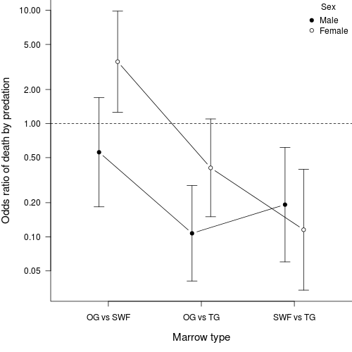
Q7-4. It appears that there are significant interactions between cause of death and bone marrow type for both females and males. Given that there was a significant interaction between cause of death and sex and bone marrow type, it is likely that the nature of the two way interactions in females is different to the two way interactions in males. To explore this further, we will examine the odds ratios for each pairwise comparison of bone marrow type with respect to predation level (for each sex)!.
Calculate the odds ratios for wildebeest killed by predation for each pair of marrow types separately for males and females

Show code

> library(epitools)

> library(biology)

> female.tab <- xtabs(COUNT ~ DEATH + MARROW, data = sinclair.split[["FEMALE"]])

> female.odds <- oddsratios(t(female.tab))

> female.odds

Comparison estimate lower upper midp.exact fisher.exact

1 OG vs SWF 3.5208333 1.26009037 9.8376018 0.0137649202 0.0206121992

2 OG vs TG 0.4062500 0.15034804 1.0977134 0.0788761506 0.0914047377

3 SWF vs TG 0.1153846 0.03378972 0.3940136 0.0003808416 0.0003765135

chi.square

1 0.0133633241

2 0.0718385552

3 0.0002797362

#Males

> library(biology)

> male.tab <- xtabs(COUNT ~ DEATH + MARROW, data = sinclair.split[["MALE"]])

> male.odds <- oddsratios(t(male.tab))

Comparison estimate lower upper midp.exact fisher.exact

1 OG vs SWF 0.5581395 0.18389618 1.6939979 3.199869e-01 3.762577e-01

2 OG vs TG 0.1073345 0.04067922 0.2832085 2.247925e-06 2.928685e-06

3 SWF vs TG 0.1923077 0.06004081 0.6159519 5.465174e-03 5.794237e-03

chi.square

1 2.998756e-01

2 1.865442e-06

3 4.123680e-03

	Odds ratio	95% CI min	95% CI max
Females
OG vs TG
SWF vs TG
SWF vs OG
Males
OG vs TG
SWF vs TG
SWF vs OG

Q7-6. The patterns revealed in the odds ratios might be easier to see, if they were presented graphically - do it.

Show code

> par(mar = c(5, 5, 0, 0))

> plot(estimate ~ as.numeric(Comparison), data = female.odds, log = "y",

> type = "n", axes = F, ann = F, ylim = range(c(upper, lower)),

> xlim = c(0.5, 3.5))

> with(female.odds, arrows(as.numeric(Comparison) + 0.1, upper,

> as.numeric(Comparison) + 0.1, lower, ang = 90, length = 0.1,

> code = 3))

> with(female.odds, points(as.numeric(Comparison) + 0.1, estimate,

> type = "b", pch = 21, bg = "white"))

> with(male.odds, arrows(as.numeric(Comparison) - 0.1, upper, as.numeric(Comparison) -

> 0.1, lower, ang = 90, length = 0.1, code = 3))

> with(male.odds, points(as.numeric(Comparison) - 0.1, estimate,

> type = "b", pch = 21, bg = "black", lty = 1))

> abline(h = 1, lty = 2)

> with(female.odds, axis(1, at = as.numeric(Comparison), lab = Comparison))

> mtext("Marrow type", 1, line = 3, cex = 1.25)

> axis(2, las = 1)

> mtext("Odds ratio of death by predation", 2, line = 4, cex = 1.25)

> legend("topright", legend = c("Male", "Female"), pch = 21, bty = "n",

> title = "Sex", pt.bg = c("black", "white"))

> box(bty = "l")

Q7-7. What would your conclusions be?

Power and continguency tables

A marine ecologist was interested in investigating whether hermit crabs on North Stradbroke Island (what a wet ecologist does on holidays I guess!). He intended to score shells according to whether or not they were occupied and whether they what type of gastropod they were from (Austrocochlea or Bembicium). Shells with living gastropods were to be ignored. Essentially, the NERD wanted to know whether or not hermit crabs occupy shells in the proportions that they are available. A quick count of shells on the rocky shore revealed that approximately 40% of available gastropod shells were occupied and that Austrocochlea or Bembicium shells were approximately equally available.
The ecologist scratched his sparsely haired scalp, raised one eyebrow and contemplated performing a quick power analysis to determine how many observation would be required to have an 80% chance of detecting a 20% preference for Austrocochlea shells.

This task is best broken down into parts.

Q8-1.
First we compile what is know about the availability of shells:

Create a variable that contains the proportion of occupied shells and another that contains the proportion of unoccupied shells (HINT, HINT).
Now create two variables that contains the proportion of Austrocochlea and Bembicium shells respectively (HINT, HINT).
Next create a table of proportions that reflect the null hypothesis situation - that is, the proportions expected when hermit crabs show no preferences at all. (HINT, HINT). Provide row (HINT) and column (HINT) titles for this table. Examine this table (HINT)
Now create a variable that contains the anticipated deviance from the null hypothesis - the proportion (20%=0.2) by which the preferences of the hermit crabs deviate from the null hypothesis (HINT).
Use this deviance to calculate the expected proportions when this alternative hypothesis (H1) is true (HINT, HINT, HINT). Examine this table (HINT)
Calculate the effect size (HINT).
Calculate appropriate degrees of freedom (HINT).
Finally, we can calculate the approximate number of total observations needed to have an 80% chance of detecting the 20% preference (HINT). How many gastropod shells need to be sampled?

Workshop 8 - Frequency analysis and generalized linear models

Basic statistics references

Goodness of fit test

Contingency tables

Download French data set

Contingency tables

Download Arrington data set

Contingency tables

Download Woodlice data set

Logistic regression

Download Polis data set

Log-linear modelling

Download Roberts data set

Log-linear modelling

Download French data set

Power and continguency tables

Welcome to the end of Workshop 8