In an unusually detailed preparation for an Environmental Effects Statement for a proposed discharge of dairy wastes into the Curdies River, in western Victoria, a team of stream ecologists wanted to describe the basic patterns of variation in a stream invertebrate thought to be sensitive to nutrient enrichment. As an indicator species, they focused on a small flatworm, Dugesia, and started by sampling populations of this worm at a range of scales. They sampled in two seasons, representing different flow regimes of the river - Winter and Summer. Within each season, they sampled three randomly chosen (well, haphazardly, because sites are nearly always chosen to be close to road access) sites. A total of six sites in all were visited, 3 in each season. At each site, they sampled six stones, and counted the number of flatworms on each stone.
The SITE variable is supposed to represent a random factorial variable (which site). However, because the contents of this variable are numbers, R initially treats them as numbers, and therefore considers the variable to be numeric rather than categorical. In order to force R to treat this variable as a factor (categorical) it is necessary to first
convert this numeric variable into a factor (HINT)
.
Show code
> curdies$SITE <- as.factor(curdies$SITE)
Notice the data set - each of the nested factors is labelled differently - there can be no replicate for the random (nesting) factor.
Q1-1. What are the main hypotheses being tested?
H0 Effect 1:
H0 Effect 2:
Q1-2. In the table below, list the assumptions of nested ANOVA along with how violations of each assumption are diagnosed and/or the risks of violations are minimized.
Assumption
Diagnostic/Risk Minimization
I.
II.
III.
Q1-3. Check these assumptions
(HINT).
Show code
> library(nlme)> curdies.ag <- gsummary(curdies, form = ~SEASON/SITE, mean)
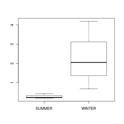
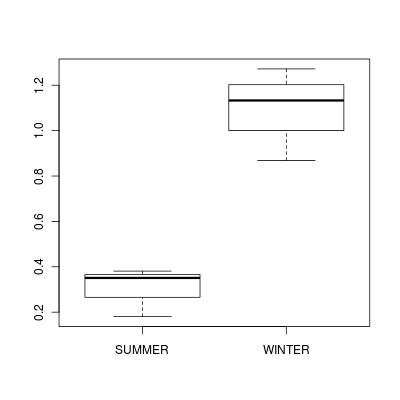
Note that for the effects of SEASON (Factor A in a nested model) there are only three values for each of the two season types.
Therefore, boxplots are of limited value! Is there however, any evidence of violations of the assumptions
(HINT)?
Show code
> boxplot(DUGESIA ~ SEASON, curdies.ag)
(Y or N) If so, assess whether a transformation will address the violations (HINT) and then make the appropriate corrections
Q1-4. For each of the tests, state which error (or residual) term (state as Mean Square) will be used as the nominator and denominator to calculate the F ratio. Also include degrees of freedom associated with each term.
Effect
Nominator (Mean Sq, df)
Denominator (Mean Sq, df)
SEASON
SITE
Q1-5. If there is no evidence of violations, test the model; S4DUGES = SEASON + SITE + CONSTANT using a nested ANOVA
(HINT).
Fill (HINT) out the table below, make sure that you have treated SITE as a random factor when compiling the overall results.
Show code
> curdies.aov <- aov(S4DUGES ~ SEASON + Error(SITE), data = curdies)> summary(curdies.aov)
Q1-6. For each of the tests, state which error (or residual) term (state as Mean Square) will be used as the nominator and denominator to calculate the F ratio. Also include degrees of freedom associated with each term.
Source of variation
df
Mean Sq
F-ratio
P-value
SEASON
SITE
Residuals
Estimate
Mean
Lower 95% CI
Upper 95% CI
Summer
Effect size (Winter-Summer)
Normally, we are not interested in formally testing the effect of the nested factor to get the correct F test for the nested factor (SITE), examine a representation of the anova table of the fitted linear model that assumes all factors are fixed (HINT)
Q1-7. What are your conclusions (statistical and biological)?
Q1-8. Now analyse these data using a linear mixed effects model (REML).
Show code - lme
> library(nlme)> curdies.lme <- lme(S4DUGES ~ SEASON, random = ~1 | SITE, data = curdies)> summary(curdies.lme)
#Calculate the confidence interval for the effect size of the main effect of season
> intervals(curdies.lme)
Approximate 95% confidence intervals
Fixed effects:
lower est. upper
(Intercept) 0.1106923 0.3041353 0.4975783
SEASONWINTER 0.4148441 0.7867589 1.1586737
attr(,"label")
[1] "Fixed effects:"
Random Effects:
Level: SITE
lower est. upper
sd((Intercept)) 1.837163e-07 0.04008598 8746.562
Within-group standard error:
lower est. upper
0.3025499 0.3896803 0.5019033
#Examine the ANOVA table with Type I (sequential) SS
> anova(curdies.lme)
numDF denDF F-value p-value
(Intercept) 1 30 108.45711 <.0001
SEASON 1 4 34.49647 0.0042
Show code - lmer
> library(lme4)> curdies.lmer <- lmer(S4DUGES ~ SEASON + (1 | SITE), data = curdies)> summary(curdies.lmer)
Linear mixed model fit by REML
Formula: S4DUGES ~ SEASON + (1 | SITE)
Data: curdies
AIC BIC logLik deviance REMLdev
46.44 52.77 -19.22 32.52 38.44
Random effects:
Groups Name Variance Std.Dev.
SITE (Intercept) 1.1647e-13 3.4127e-07
Residual 1.5299e-01 3.9113e-01
Number of obs: 36, groups: SITE, 6
Fixed effects:
Estimate Std. Error t value
(Intercept) 0.30414 0.09219 3.299
SEASONWINTER 0.78676 0.13038 6.034
Correlation of Fixed Effects:
(Intr)
SEASONWINTE -0.707
#Calculate the confidence interval for the effect size of the main effect of season
> library(languageR)> pvals.fnc(curdies.lmer, withMCMC = FALSE, addPlot = F)
Groups Name Std.Dev. MCMCmedian MCMCmean HPD95lower HPD95upper
1 SITE (Intercept) 0.0000 0.0562 0.0827 0.0000 0.2652
2 Residual 0.3911 0.3878 0.3928 0.3032 0.4922
#Examine the effect season via a likelihood ratio test
> curdies.lmer1 <- lmer(S4DUGES ~ SEASON + (1 | SITE), data = curdies, > REML = F)> curdies.lmer2 <- lmer(S4DUGES ~ 1 + (1 | SITE), data = curdies, > REML = F)> anova(curdies.lmer1, curdies.lmer2, test = "F")
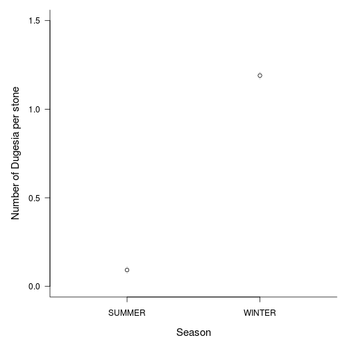
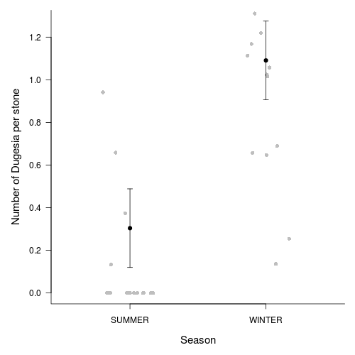
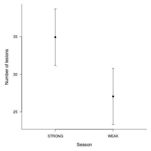
Plot predicted mean transformed number of Dugesia (and confidence interval) for each season.
Note that these data were modelled with a Gaussian distribution (this might not have been appropriate)
Show code
> newdata[, -1] <- newdata[, -1]^4> par(mar = c(5, 5, 1, 1))> plot(S4DUGES ~ as.numeric(SEASON), newdata, type = "n", axes = F, > ann = F, ylim = range(newdata$plo, newdata$phi), xlim = c(0.5, > 2.5))> points(curdies$DUGESIA ~ jitter(as.numeric(curdies$SEASON)), > pch = 16, col = "grey")> with(newdata, arrows(as.numeric(SEASON), plo, as.numeric(SEASON), > phi, ang = 90, length = 0.05, code = 3))> with(newdata, points(as.numeric(SEASON), S4DUGES, pch = 21, bg = "black", > col = "black"))> axis(1, at = c(1, 2), lab = newdata$SEASON)> axis(2, las = 1)> mtext("Number of Dugesia per stone", 2, line = 3, cex = 1.25)> mtext("Season", 1, line = 3, cex = 1.25)> box(bty = "l")
Note, backtransforming the standard deviations has the reverse effect to desired (since they are less than 1).
Q1-10. How might this information influence the design of future experiments on Dugesia in terms of:
What influences the abundance of Dugesia
Where best to focus sampling effort to maximize statistical power?
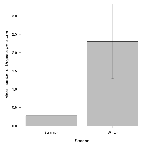
Q1-11.Finally, construct an appropriate summary figure
to accompany the above analyses. Note that this should use the correct replicates for depicting error.
Show code
> opar <- par(mar = c(5, 5, 1, 1))> means <- tapply(curdies.ag$DUGESIA, curdies.ag$SEASON, mean)> sds <- tapply(curdies.ag$DUGESIA, curdies.ag$SEASON, sd)> lens <- tapply(curdies.ag$DUGESIA, curdies.ag$SEASON, length)> ses <- sds/sqrt(lens)> xs <- barplot(means, beside = T, ann = F, axes = F, ylim = c(0, > max(means + ses)), axisnames = F)> arrows(xs, means - ses, xs, means + ses, code = 3, length = 0.05, > ang = 90)> axis(1, at = xs, lab = c("Summer", "Winter"))> mtext("Season", 1, line = 3, cex = 1.25)> axis(2, las = 1)> mtext("Mean number of Dugesia per stone", 2, line = 3, cex = 1.25)> box(bty = "l")
A plant pathologist wanted to examine the effects of two different strengths of tobacco virus on the number of lesions on tobacco leaves. She knew from pilot studies that leaves were inherently very variable in response to the virus. In an attempt to account for this leaf to leaf variability, both treatments were applied to each leaf. Eight individual leaves were divided in half, with half of each leaf inoculated with weak strength virus and the other half inoculated with strong virus. So the leaves were blocks and each treatment was represented once in each block. A completely randomised design would have had 16 leaves, with 8 whole leaves randomly allocated to each treatment.
Since each level of treatment was applied to each leaf, the data represents a randomized block design with leaves as blocks.
The variable LEAF contains a list of Leaf identification numbers and is supposed to represent a factorial blocking variable.
However, because the contents of this variable are numbers, R initially treats them as numbers, and therefore considers the variable to be numeric rather than categorical.
In order to force R to treat this variable as a factor (categorical) it is necessary to first
convert this numeric variable into a factor
(HINT).
Show code
> tobacco$LEAF <- as.factor(tobacco$LEAF)
Q2-1. What are the main hypotheses being tested?
H0 Factor A:
H0 Factor B:
Q2-2. In the table below, list the assumptions of a randomized block design along with how violations of each assumption are diagnosed and/or the risks of violations are minimized.
Assumption
Diagnostic/Risk Minimization
I.
II.
III.
IV.
Is the proposed model
balanced?
(Yor N)
Show code
> replications(NUMBER ~ LEAF + TREATMENT, data = tobacco)
LEAF TREATMENT
2 8
> !is.list(replications(NUMBER ~ LEAF + TREATMENT, data = tobacco))
[1] TRUE
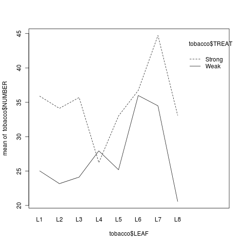
Q2-3. There are a number of
ways of diagnosing block by within block interactions.
The simplest method is to plot the number of lesions for each treatment and leaf combination (ie. an
interaction plot
(HINT). Any evidence of an interaction? Note that we cannot formally test for an interaction because we don't have replicates for each treatment-leaf combination!
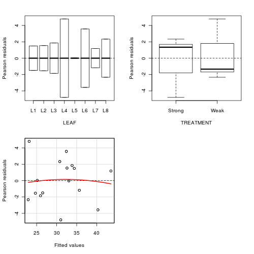
We can also examine the residual plot from the fitted linear
model. A curvilinear pattern in which the residual values switch from positive to negative
and back again (or visa versa) over the range of predicted values implies that the scale
(magnitude but not polarity) of the main treatment effects differs substantially across the range
of blocks. (HINT). Any evidence of an interaction?
Show code
> residualPlots(lm(NUMBER ~ LEAF + TREATMENT, data = tobacco))
Test stat Pr(>|t|)
LEAF NA NA
TREATMENT NA NA
Tukey test -0.18 0.858
Perform a Tukey's test for non-additivity evaluated at α = 0.10 or even &alpha = 0.25. This (curvilinear test)
formally tests for the presence of a quadratic trend in the relationship between residuals and
predicted values. As such, it too is only appropriate for simple interactions of scale.
(HINT). Any evidence of an interaction?
Show code
> library(alr3)> tukey.nonadd.test(lm(NUMBER ~ LEAF + TREATMENT, data = tobacco))
Test Pvalue
-0.1795228 0.8575272
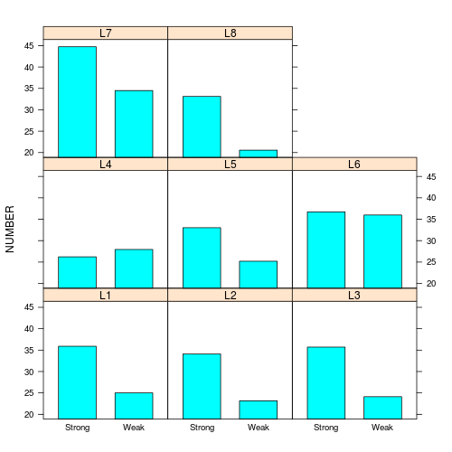
Examine a lattice graphic to determine the consistency of the
effect across each of the blocks(HINT).
Show code
> library(lattice)> print(barchart(NUMBER ~ TREATMENT | LEAF, data = tobacco))
Q2-4. Analyse these data with a classic
randomized block ANOVA
(HINT) to test the H0 that there is no difference in the number of lesions produced by the different strength viruses. Complete the table below.
#Calculate the confidence interval for the effect size of the main effect of season
> library(languageR)> pvals.fnc(tobacco.lmer, withMCMC = FALSE, addPlot = F)
In an attempt to understand the effects on marine animals of short-term exposure to toxic substances, such as might occur following a spill, or a major increase in storm water flows, a it was decided to examine the toxicant in question, Copper, as part of a field experiment in Honk Kong. The experiment consisted of small sources of Cu (small, hemispherical plaster blocks, impregnated with copper), which released the metal into sea water over 4 or 5 days. The organism whose response to Cu was being measured was a small, polychaete worm, Hydroides, that attaches to hard surfaces in the sea, and is one of the first species to colonize any surface that is submerged. The biological questions focused on whether the timing of exposure to Cu affects the overall abundance of these worms. The time period of interest was the first or second week after a surface being available.
The experimental setup consisted of sheets of black perspex (settlement plates), which provided good surfaces for these worms. Each plate had a plaster block bolted to its centre, and the dissolving block would create a gradient of [Cu] across the plate. Over the two weeks of the experiment, a given plate would have pl ain plaster blocks (Control) or a block containing copper in the first week, followed by a plain block, or a plain block in the first week, followed by a dose of copper in the second week. After two weeks in the water, plates were removed and counted back in the laboratory. Without a clear idea of how sensitive these worms are to copper, an effect of the treatments might show up as an overall difference in the density of worms across a plate, or it could show up as a gradient in abundance across the plate, with a different gradient in different treatments. Therefore, on each plate, the density of worms (#/cm2) was recorded at each of four distances from the center of the plate.
Categorical listing of the copper treatment (control = no copper applied, week 2 = copper treatment applied in second week and week 1= copper treatment applied in first week) applied to whole plates. Factor A (between plot factor).
PLATE
Substrate provided for polychaete worm colonization on which copper treatment applied. These are the plots (Factor B). Numbers in this column represent numerical labels given to each plate.
DIST
Categorical listing for the four concentric distances from the center of the plate (source of copper treatment) with 1 being the closest and 4 the furthest. Factor C (within plot factor)
WORMS
Density (#/cm2) of worms measured. Response variable.
Q3-2. The usual ANOVA assumptions apply to split-plot designs, and these can be tested by constructing boxplots for each of the main effects. However, it is important to consider what data the boxplots should be based upon. For each of the main hypothesis tests, describe what data should be used to construct boxplots (remember that the assumptions of normality and homogeneity of variance apply to the residuals of each hypothesis test, and therefore the data used in the construction of boxplots for each hypothesis test should represent the respective residuals, or sources of unexplained variation).
H0 Main Effect 1 (Factor A):
H0 Main Effect 2 (Factor C):
H0 Main Effect 3 (A*C):
Q3-3. For each of the hypothesis tests, indicate which Mean Square term should be used as the residual (denominator) in the F-ratio calculation. Note, COPPER and DIST are fixed factors and PLATE is a random factor.
H0 Main Effect 1 (Factor A): F-ratio = MSCOPPER/MS
H0 Main Effect 2 (Factor C): F-ratio = MSDIST/MS
H0 Main Effect 3 (A*C): F-ratio = MSCOPPER:DIST/MS
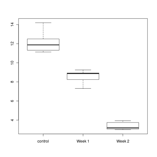
Q3-4. Construct a boxplot to investigate the assumptions as they apply to the test of H0 Main Effect 1 (Factor A): This is done in two steps
Aggregate the data set by the mean number of WORMS within each plate
(HINT)
Construct a boxplot of aggregated mean number of WORMS against COPPER treatment
(HINT)
Show code
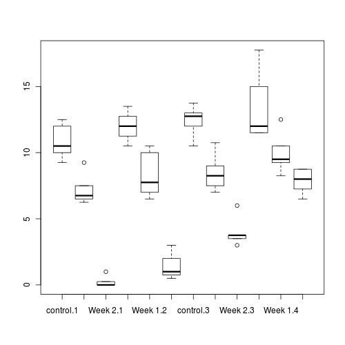
> boxplot(WORMS ~ COPPER, data = cu.ag)
Any evidence of violations of the assumptions (y or n)?
Q3-5.
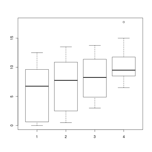
Construct a boxplot to investigate the assumptions as they apply to the test of H0 Main Effect 2 (Factor C): Since Factor C is tested against the overal residual in this case, this is a relatively straight forward procedure.
(HINT)
Show code
> boxplot(WORMS ~ DIST, data = copper)
Any evidence of violations of the assumptions (y or n)?
Q3-6.
Construct a boxplot to investigate the assumptions as they apply to the test of H0 the main interaction effect (A:C): Since A:C is tested against the overal residual, this is a relatively straight forward procedure.(HINT)
Show code
> boxplot(WORMS ~ COPPER:DIST, data = copper)
Any evidence of violations of the assumptions (y or n)?
Q3-7.
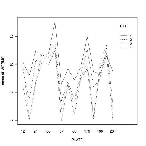
In addition to the above assumptions, the test of PLATE assumes that there is no PLATE by DIST interaction as this is the overal residual (the replicates).
That is, the test assumes that the effect of DIST is consistent in all PLATES.
Construct an interaction plot to examine whether there is any evidence of an interaction between PLATE and DISTANCE
(HINT)
Q3-9. Perform a
split-plot ANOVA
(HINT),
and complete the following table (HINT).
To obtain the hypothesis test for the random factor (Factor B: PLATE), run the model as if all factors were fixed and thus all terms are tested against the overall residuals,
HINT)
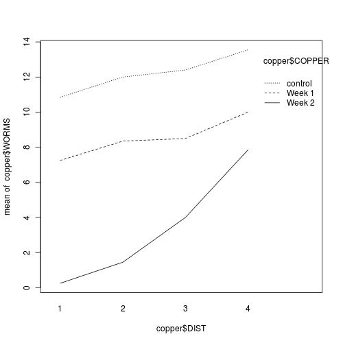
Q3-10.Construct an
interaction plot
showing the density of worms against distance from Cu source, with each treatment as different lines (or different bars).
HINT
Q3-11. What conclusions would you draw from the analysis (and graph)?
Q3-12.
In order to tease out the interaction, we could analyse the effects of the main factor (COPPER) separately for each Distance and/or investigate the effects of Distance separately for each of the three copper treatments.
Recall that when performing such simple main effects, it is necessary to use the residual terms from the global analyses as these are likely to be better estimates (as they are based on a larger amount of data).
Investigate the effects of copper separately for each of the
four distances HINT
Show code
> AnovaM(mainEffects(copper.aov, at = DIST == 1), type = "III")
Check whether a first order autoregressive correlation structure is more appropriate
> copper.lme2 <- update(copper.lme, correlation = corAR1(form = ~1 | > PLATE))> anova(copper.lme, copper.lme2)
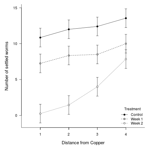
Broad interpretation:
In general, compared to the number of worms settling on the control plates, the number of worms settling was less in the Week 1 treatment and even lower in the Week 2 treatment.
The increases in number of settled worms in distances progressively further from the source (Dist 1) get progressively larger
and the trend between DIST1 (base level) and DIST 4 is significantly greater for the Week 2 treatment compared to the control copper treatment.
Examine the model fit measures
Show code
> summary(copper.lmer)@AICtab
AIC BIC logLik deviance REMLdev
218.2515 247.5723 -95.12575 200.2842 190.2515
Examine the variance components
Show code
> data.frame(summary(copper.lmer)@REmat)
Groups Name Variance Std.Dev.
1 PLATE (Intercept) 0.31354 0.55995
2 Residual 1.80677 1.34416
Examine the predicted means and confidence intervals
Interpretation: Compared to the number of worms settling on control plates, the number of settling worms is less in Week 1 and even lower in the Week 2 copper treatment.
Settlement increases with increasing distance from the copper source and this rate of increase is over twice the rate (significantly greater) in the Week 2 treatment.
Show code - ezAnova
> library(ez)> ezANOVA(dv = .(WORMS), between = .(COPPER), within = .(DIST), > wid = .(PLATE), data = copper, type = 3)
In an honours thesis from (1992), Mullens was investigating the ways that cane toads ( Bufo marinus ) respond to conditions of hypoxia. Toads show two different kinds of breathing patterns, lung or buccal, requiring them to be treated separately in the experiment. Her aim was to expose toads to a range of O2 concentrations, and record their breathing patterns, including parameters such as the expired volume for individual breaths. It was desirable to have around 8 replicates to compare the responses of the two breathing types, and the complication is that animals are expensive, and different individuals are likely to have different O2 profiles (leading to possibly reduced power). There are two main design options for this experiment;
One animal per O2 treatment, 8 concentrations, 2 breathing types. With 8 replicates the experiment would require 128 animals, but that this could be analysed as a completely randomized design
One O2 profile per animal, so that each animal would be used 8 times and only 16 animals are required (8 lung and 8 buccal breathers)
Mullens decided to use the second option so as to reduce the number of animals required (on financial and ethical grounds). By selecting this option, she did not have a set of independent measurements for each oxygen concentration, by repeated measurements on each animal across the 8 oxygen concentrations.
Categorical listing of the breathing type treatment (buccal = buccal breathing toads, lung = lung breathing toads). This is the between subjects (plots) effect and applies to the whole toads (since a single toad can only be one breathing type - either lung or buccal). Equivalent to Factor A (between plots effect) in a split-plot design
TOAD
These are the subjects (equivalent to the plots in a split-plot design: Factor B). The letters in this variable represent the labels given to each individual toad.
O2LEVEL
0 through to 50 represent the the different oxygen concentrations (0% to 50%). The different oxygen concentrations are equivalent to the within plot effects in a split-plot (Factor C).
FREQBUC
The frequency of buccal breathing - the response variable
SFREQBUC
Square root transformed frequency of buccal breathing - the response variable
Notice that both the O2LEVEL variable contains only numbers. Make sure that you define both of this as a factors (HINT)
Show code
> mullens$O2LEVEL <- factor(mullens$O2LEVEL)
Q4-1. What are the main hypotheses being tested?
H0 Main Effect 1 (Factor A):
H0 Main Effect 2 (Factor C):
H0 Main Effect 3 (A*C):
Q4-2. We will now address all the assumptions.
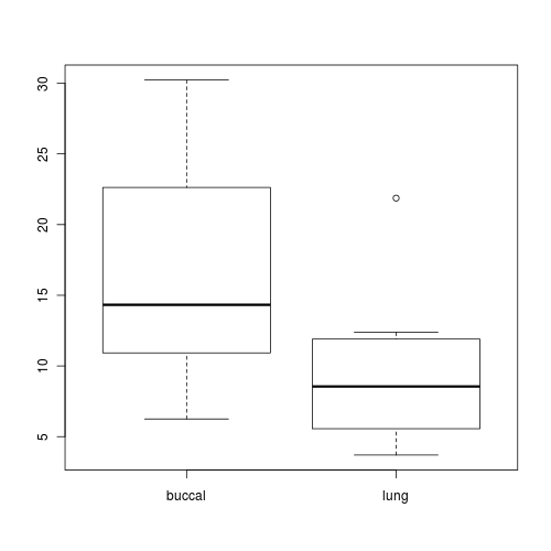
Construct a boxplot to investigate the assumptions as they apply to the test of H0 Main Effect 1 (Factor A): This is done in two steps
Construct a boxplot to investigate the assumptions as they apply to the test of H0 Main Effect 1 (Factor A):
Start by aggregating the data set by TOAD
(since the toads are the replicates for the between subject effect - BREATH) (HINT).
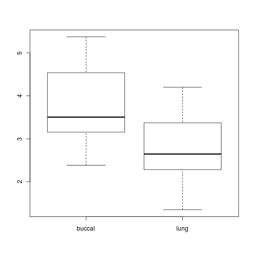
Then Construct a boxplot of aggregated mean FREQBUC against BREATH treatment
(HINT).
Any evidence of violations of the assumptions (y or n)?
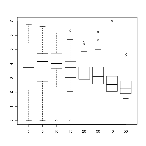
Construct a boxplot to investigate the assumptions as they apply to the test of H0 Main Effect 2 (Factor C): Since Factor C is tested against the overall residual in this case, this is a relatively straight forward procedure.(HINT).
Any evidence of violations of the assumptions (y or n)?
Show code
> boxplot(SFREQBUC ~ O2LEVEL, mullens)
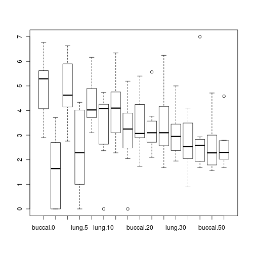
Construct a boxplot to investigate the assumptions as they apply to the test of H0 the main interaction effect (A:C): Since A:C is tested against the overal residual, this is a relatively straight forward procedure.(HINT).
Any evidence of violations of the assumptions (y or n)?
Show code
> boxplot(SFREQBUC ~ BREATH * O2LEVEL, mullens)
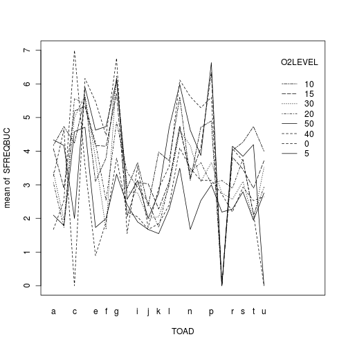
In addition to the above assumptions, the test of TOAD assumes that there is no TOAD by O2LEVEL interaction as this is the overal residual (the replicates).
That is, the test assumes that the effect of O2LEVEL is consistent in all TOADS.
Construct an interaction plot to examine whether there is any evidence of an interaction between TOAD and O2LEVEL
(HINT).
Any evidence of an interaction (y or n)?
Q4-3. Assume that the assumption of compound symmetry/sphericity will be violated and perform a
split-plot ANOVA (repeated measures)
(HINT),
and complete the following table with corrected p-values (HINT).
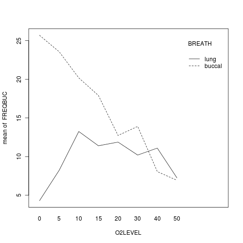
Q4-4.
Construct an interaction plot
showing the frequency of buccal breathing against oxygen level, with each breathing type as different lines (or different bars).
HINT