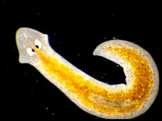
In an unusually detailed preparation for an Environmental Effects Statement for a proposed discharge of dairy wastes into the Curdies River, in western Victoria, a team of stream ecologists wanted to describe the basic patterns of variation in a stream invertebrate thought to be sensitive to nutrient enrichment. As an indicator species, they focused on a small flatworm, Dugesia, and started by sampling populations of this worm at a range of scales. They sampled in two seasons, representing different flow regimes of the river - Winter and Summer. Within each season, they sampled three randomly chosen (well, haphazardly, because sites are nearly always chosen to be close to road access) sites. A total of six sites in all were visited, 3 in each season. At each site, they sampled six stones, and counted the number of flatworms on each stone.
The SITE variable is supposed to represent a random factorial variable (which site). However, because the contents of this variable are numbers, R initially treats them as numbers, and therefore considers the variable to be numeric rather than categorical. In order to force R to treat this variable as a factor (categorical) it is necessary to first
convert this numeric variable into a factor (HINT)
.
Show code
> curdies$SITE <- as.factor(curdies$SITE)
Notice the data set - each of the nested factors is labelled differently - there can be no replicate for the random (nesting) factor.
Q1-1. What are the main hypotheses being tested?
H0 Effect 1:
H0 Effect 2:
Q1-2. In the table below, list the assumptions of nested ANOVA along with how violations of each assumption are diagnosed and/or the risks of violations are minimized.
Assumption
Diagnostic/Risk Minimization
I.
II.
III.
Q1-3. Check these assumptions
(HINT).
Show code
> library(nlme)> curdies.ag <- gsummary(curdies, form = ~SEASON/SITE, mean)
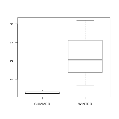
Note that for the effects of SEASON (Factor A in a nested model) there are only three values for each of the two season types.
Therefore, boxplots are of limited value! Is there however, any evidence of violations of the assumptions
(HINT)?
Show code
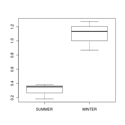
> boxplot(DUGESIA ~ SEASON, curdies.ag)
(Y or N) If so, assess whether a transformation will address the violations (HINT) and then make the appropriate corrections
Q1-4. For each of the tests, state which error (or residual) term (state as Mean Square) will be used as the nominator and denominator to calculate the F ratio. Also include degrees of freedom associated with each term.
Effect
Nominator (Mean Sq, df)
Denominator (Mean Sq, df)
SEASON
SITE
Q1-5. If there is no evidence of violations, test the model; S4DUGES = SEASON + SITE + CONSTANT using a nested ANOVA
(HINT).
Fill (HINT) out the table below, make sure that you have treated SITE as a random factor when compiling the overall results.
Show code
> curdies.aov <- aov(S4DUGES ~ SEASON + Error(SITE), data = curdies)> summary(curdies.aov)
F-statistic: 8.188 on 5 and 30 DF, p-value: 5.718e-05
> confint(lm(curdies.aov))
2.5 % 97.5 %
(Intercept) 0.05622464 0.7060200
SEASONWINTER 0.29234513 1.2112945
SITE2 -0.32054693 0.5984024
SITE3 -0.72454609 0.1944033
SITE4 -0.48977564 0.4291737
SITE5 -0.66013474 0.2588146
SITE6 NA NA
Q1-6. For each of the tests, state which error (or residual) term (state as Mean Square) will be used as the nominator and denominator to calculate the F ratio. Also include degrees of freedom associated with each term.
Source of variation
df
Mean Sq
F-ratio
P-value
SEASON
SITE
Residuals
Estimate
Mean
Lower 95% CI
Upper 95% CI
Summer
Effect size (Winter-Summer)
Normally, we are not interested in formally testing the effect of the nested factor to get the correct F test for the nested factor (SITE), examine a representation of the anova table of the fitted linear model that assumes all factors are fixed (HINT)
Q1-7. What are your conclusions (statistical and biological)?
Q1-8. Where is the major variation in numbers of flatworms? Between (seasons, sites or stones)?
Q1-9. How might this information influence the design of future experiments on Dugesia in terms of:
What influences the abundance of Dugesia
Where best to focus sampling effort to maximize statistical power?
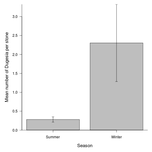
Q1-10.Finally, construct an appropriate summary figure
to accompany the above analyses. Note that this should use the correct replicates for depicting error.
Show code
> opar <- par(mar = c(5, 5, 1, 1))> means <- tapply(curdies.ag$DUGESIA, curdies.ag$SEASON, mean)> sds <- tapply(curdies.ag$DUGESIA, curdies.ag$SEASON, sd)> lens <- tapply(curdies.ag$DUGESIA, curdies.ag$SEASON, length)> ses <- sds/sqrt(lens)> xs <- barplot(means, beside = T, ann = F, axes = F, ylim = c(0, > max(means + ses)), axisnames = F)> arrows(xs, means - ses, xs, means + ses, code = 3, length = 0.05, > ang = 90)> axis(1, at = xs, lab = c("Summer", "Winter"))> mtext("Season", 1, line = 3, cex = 1.25)> axis(2, las = 1)> mtext("Mean number of Dugesia per stone", 2, line = 3, cex = 1.25)> box(bty = "l")
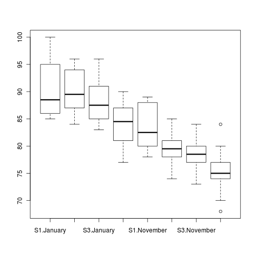
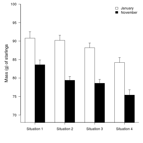
A biologist studying starlings wanted to know whether the mean mass of starlings differed according to different roosting situations. She was also interested in whether the mean mass of starlings altered over winter (Northern hemisphere) and whether the patterns amongst roosting situations were consistent throughout winter, therefore starlings were captured at the start (November) and end of winter (January). Ten starlings were captured from each roosting situation in each season, so in total, 80 birds were captured and weighed.
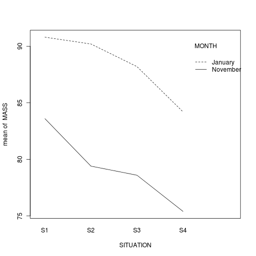
In the classical frequentist regime, many at this point would advocate dropping the interaction term from the model (p-value for the interaction is greater than 0.25).
This term is not soaking up much of the residual and yet is soaking up 3 degrees of freedom. The figure also indicates that situation and month are likely to operate additively.
Q2-5. In the absence of an interaction, we can examine the effects of each of the main effects in isolation.
It is not necessary to examine the effect of MONTH any further, as there were only two groups.
However, if we wished to know which roosting situations were significantly different to one another, we need to perform additional
multiple comparisons
. Since we don't know anything about the roosting situations, no one comparison is any more or less meaningful than any other comparisons. Therefore, a Tukey's test is most appropriate. Perform a
Tukey's test (HINT)
and summarize indicate which of the following comparisons were significant (put * in the box to indicate P< 0.05, ** to indicate P< 0.001, and NS to indicate not-significant).
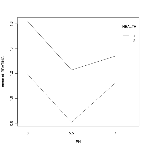
Here is a modified example from Quinn and Keough (2002). Stehman and Meredith (1995) present data from an experiment that was set up to test the hypothesis that
healthy spruce seedlings break bud sooner than diseased spruce seedlings. There were 2 factors: pH (3
levels: 3, 5.5, 7) and HEALTH (2 levels: healthy, diseased). The dependent variable was the average
(from 5 buds) bud emergence rating (BRATING) on each seedling. The sample size varied for each
combination of pH and health, ranging from 7 to 23 seedlings. With two factors, this experiment should
be analyzed with a 2 factor (2 x 3) ANOVA.
Categorical listing of pH (not however that the levels are numbers and thus by default the variable is treated as a numeric variable rather than a factor - we need to correct for this)
HEALTH
Categorical listing of the health status of the seedlings, D = diseased, H = healthy
GROUP
Categorical listing of pH/health combinations - used for checking ANOVA assumptions
The variable PH contains a list of pH values and is supposed to represent a factorial variable.
However, because the contents of this variable are numbers, R initially treats them as numbers, and therefore considers the variable to be numeric rather than categorical. In order to force R to treat this variable as a factor (categorical) it is necessary to first
convert this numeric variable into a factor
(HINT).
Show code
> stehman$PH <- as.factor(stehman$PH)
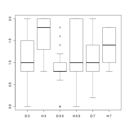
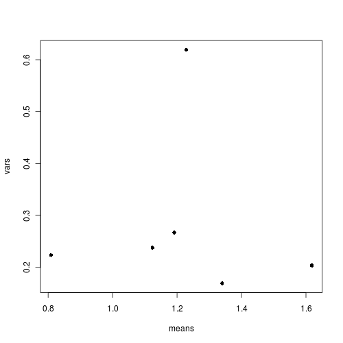
Q3-1. Test the assumptions
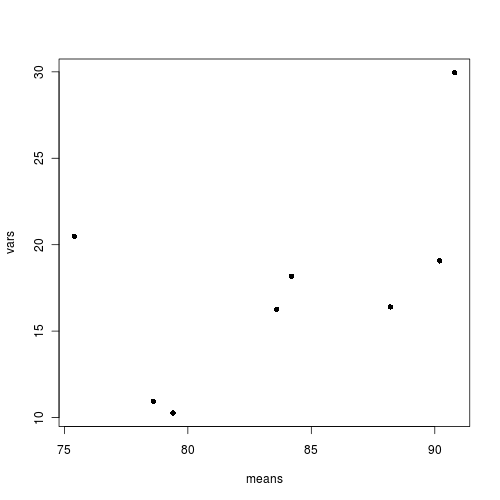
by producing boxplots
and mean vs variance plot.
Show code
> boxplot(BRATING ~ HEALTH * PH, data = stehman)
> means <- with(stehman, tapply(BRATING, list(HEALTH, PH), mean))> vars <- with(stehman, tapply(BRATING, list(HEALTH, PH), var))> plot(means, vars, pch = 16)
Is there any evidence that one or more of the assumptions are likely to be violated? (Y or N)
Is the proposed model balanced?
(Y or N)
Show code
> replications(BRATING ~ HEALTH * PH, data = stehman)
$HEALTH
HEALTH
D H
67 28
$PH
PH
3 5.5 7
34 30 31
$`HEALTH:PH`
PH
HEALTH 3 5.5 7
D 23 23 21
H 11 7 10
> !is.list(replications(BRATING ~ HEALTH * PH, data = stehman))
[1] FALSE
As the model is not balanced, we will likely want to examine the ANOVA table based on Type III (marginal) Sums of Squares.
In preparation for doing so, we must define something other than treatment contrasts for the factors.
Q3-2. Now
fit a two-factor ANOVA model
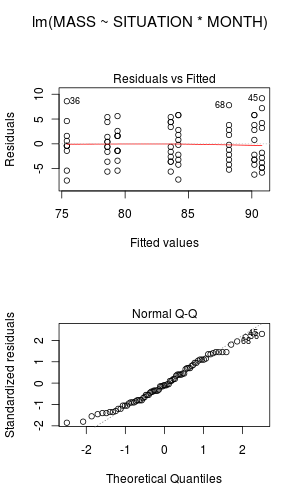
and examine the residuals.
Any evidence of skewness or unequal variances? Any outliers? Any evidence of violations? ('Y' or 'N')
.
As the model is not balanced, we will base hypothesis tests on Type II sums of squares.
Produce an ANOVA table (HINT) and fill in the following table:
Show code
> stehman.lm <- lm(BRATING ~ HEALTH * PH, data = stehman)> library(car)> Anova(stehman.lm, type = "III")
Q3-4. In the absence of an interaction, we can examine the effects of each of the main effects in isolation. It is not necessary to examine the effect of HEALTH any further, as there were only two groups. However, if we wished to know which pH levels were significantly different to one another, we need to perform additional
multiple comparisons.
Since no one comparison is any more or less meaningful than any other comparisons, a Tukey's test is most appropriate. Perform a
Tukey's test
(Adjusted p values reported -- single-step method)
and summarize indicate which of the following comparisons were significant (put * in the box to indicate P< 0.05, ** to indicate P< 0.001, and NS to indicate not-significant). pH 3 vs pH 5.5 pH 3 vs pH 7 pH 5.5 vs pH 7
Q3-5.Generate a bargraph to summarize the findings of
the above Tukey's test.
The above analysis reflects a very classic approach to investigating the effects of PH and HEALTH via NHST (null hypothesis testing).
Many argue that a more modern/valid approach is to:
Abandon hypothesis testing
Estimate effect sizes and associated effect sizes
As PH is an ordered factor, this is arguably better modelled via polynomial contrasts
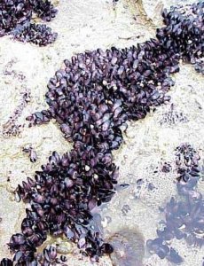
An ecologist studying a rocky shore at Phillip Island, in southeastern Australia, was interested in how
clumps of intertidal mussels are maintained. In particular, he wanted to know how densities of adult
mussels affected recruitment of young individuals from the plankton. As with most marine invertebrates,
recruitment is highly patchy in time, so he expected to find seasonal variation, and the interaction
between season and density - whether effects of adult mussel density vary across seasons - was the aspect
of most interest.
The data were collected from four seasons, and with two densities of adult mussels. The experiment
consisted of clumps of adult mussels attached to the rocks. These clumps were then brought back to the
laboratory, and the number of baby mussels recorded. There were 3-6 replicate clumps for each density
and season combination.
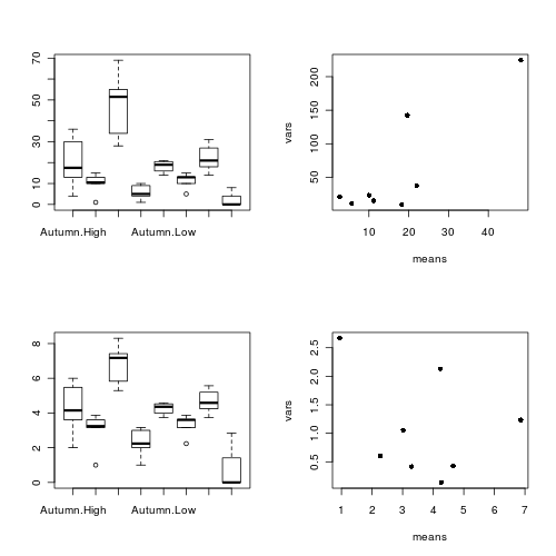
Confirm the need for a square root transformation, by examining
boxplots
and mean vs variance plots
for both raw and transformed data. Note that square root transformation was selected because the data were counts (count data often includes values of zero - cannot compute log of zero).
Show code
> par(mfrow = c(2, 2))> boxplot(RECRUITS ~ SEASON * DENSITY, data = quinn)> means <- with(quinn, tapply(RECRUITS, list(SEASON, DENSITY), > mean))> vars <- with(quinn, tapply(RECRUITS, list(SEASON, DENSITY), var))> plot(means, vars, pch = 16)> boxplot(SQRTRECRUITS ~ SEASON * DENSITY, data = quinn)> means <- with(quinn, tapply(SQRTRECRUITS, list(SEASON, DENSITY), > mean))> vars <- with(quinn, tapply(SQRTRECRUITS, list(SEASON, DENSITY), > var))> plot(means, vars, pch = 16)
Also confirm that the design (model) is unbalanced
and thus warrants the use of Type III sums of squares. (HINT)
Show code
> !is.list(replications(sqrt(RECRUITS) ~ SEASON * DENSITY, data = quinn))
[1] FALSE
> replications(sqrt(RECRUITS) ~ SEASON * DENSITY, data = quinn)
Q4-1. Now
fit a two-factor ANOVA model
(using the square-root transformed data and
examine the residuals.
Any evidence of skewness or unequal variances? Any outliers? Any evidence of violations? ('Y' or 'N') .
Produce an anova table based on Type III SS and fill in the following table:
Show code
> quinn.lm <- lm(SQRTRECRUITS ~ SEASON * DENSITY, data = quinn)> library(car)> Anova(quinn.lm, type = "III")
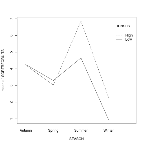
Q4-2.Summarize these trends using a
interaction plot.
Note that graphs do not place the
restrictive assumptions on data sets that formal analyses do (since graphs are
not statistical analyses). Therefore, it data transformations were used for the
purpose of meeting test assumptions, it is usually better to display raw data
(non transformed) in graphical presentations. This way readers can easily
interpret actual values in a scale that they are more familiar
with.
Q4-3. The presence of a significant interaction means that we cannot make general statements about the effect of one factor (such as density) in isolation of the other factor (e.g. season). Whether there is an effect of density depends on which season you are considering (and vice versa). One way to clarify an interaction is to analyze subsets of the data. For example, you could examine the effect of density separately at each season (using four, single factor ANOVA's), or analyze the effect of season separately (using two, single factor ANOVA's) at each mussel density.
For the current data set, the effect of density is of greatest interest, and thus the former option is the most interesting. Perform the
simple main effects anovas.