Contrasts

9 June 2011

Context

• Recent statistical advice has progressively advocated the use of effect sizes and confidence intervals over the traditional p-values of hyothesis tests.
• It is argued that the size of p-values are regularly incorrectly inferred to represent the strength of an effect.
• Proponents argue that effect sizes (the magnitude of the differences between treatment levels or trajectories) and associated measures of confidence or precision of these estimates provide far more informative summaries.
• Furthermore, the resolve of these recommendations is greatly enhanced as model complexity increases (particularly with the introduction of nesting or repeated measures) and appropriate degrees of freedom on which to base p-value calculations become increasingly more tenuous.
• Consequently, there have been numerous pieces of work that oppose/criticize/impugn the use of p-values and advocate the use of effect sizes.
• Unfortunately, few offer much guidance in how such effects sizes can be calculated, presented and interpreted.
• Therefore, the reader is left questioning the way that they perform and present their statistical findings and is confused about how they should proceed in the future knowing that if they continue to present their results in the traditional framework, they are likely to be challenged during the review process.
• This paper aims to address these issues by illustrating the following:
  • The use of contrast coefficients to calculate effect sizes, marginal means and associated confidence intervals for a range of common statistical designs.
  • The techniques apply equally to models of any complexity and model fitting procedure (including Bayesian models).
  • Graphical presentation of effect sizes
  • All examples are backed up with full R code (in appendix)

All of the following data sets are intentionally artificial. By creating data sets with specific characteristics (samples drawn from exactly known populations), we can better assess the accuracy of the techniques.

Contrasts in prediction in regression analyses

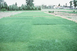
Imagine a situation in which we had just performed simple linear regression, and now we wished to summarize the trend graphically. For this demonstration, we will return to a dataset we used in a previous Workshop (the fertilizer data set): An agriculturalist was interested in the effects of fertilizer load on the yield of grass. Grass seed was sown uniformly over an area and different quantities of commercial fertilizer were applied to each of ten 1 m² randomly located plots. Two months later the grass from each plot was harvested, dried and weighed. The data are in the file fertilizer.csv.

Download Fertilizer data set

Format of fertilizer.csv data files
FERTILIZER YIELD 25 84 50 80 75 90 100 154 125 148 ... ... FERTILIZER Mass of fertilizer (g.m-2) - Predictor variable YIELD Yield of grass (g.m-2) - Response variable

Open the fertilizer dataset

Linear model parameterization for regression looks like:

yi = β0 + βi x1 + εi
εi ∼ Normal(0,σ2)	#Residual 'random' effects

Lets fit the linear model relating grass yield to fertilizer concentration:

When we fit a linear model, we estimate the values of the parameters (β₀ and β₁) such that the deviations in the predicted values of y_i are minimized (OLS). Once we have the estimates of the intercept and slope parameters, we can solve the equation for new values of x so as to predict new values of y.

For example, if the estimated intercept (β₀) and slope (β₀) where 2 and 3 respectively

, we could predict a new value of y when x was equal to 5.

yi = β0 + β1 xi

yi = 2 + 3× xi

y = 2 + 3× 5

y = 17

In other words, what we are saying, is that to estimate a new value of y, we want to add one unit of 2 to five units of 3. So the contrasts associated with predicting a new value of y from a new x value of 5 would be 1 and 5

So what we are after is what is called the outer product of the two matrices. The outer product multiplies the first entry of the left matrix by the first value (first row) of the second matrix and the second values together and so on, and then sums them all up. In R, the outer product of two matrices is performed by the %*%.

In this way, we can predict multiple new y values from multiple new x values. When the second matrix contains multiple columns, each column represents a separate contrast. Therefore the outer products are performed separately for each column of the second (contrast) matrix.

Use the predict() function to extract the line of best fit and standard errors

For simple examples such as this, there is a function called predict() that can be used to derive estimates (and standard errors) from simple linear models. This function is essentially a clever wrapper for the series of actions that we will perform manually. As it is well tested under simple conditions, it provides a good comparison and reference point for our manual calculations.

Use these predicted values to draw a line of best fit and standard error (and confidence) bands

Use contrasts and matrix algebra to derive predictions and errors

1. First retrieve the fitted model parameters (intercept and slope)

   > coefs <- fert.lm$coef

   > coefs

   (Intercept)  FERTILIZER 

    51.9333333   0.8113939 

2. Generate a model matrix appropriate for the predictor variable range. The more numbers there are over the range the smoother (less jagged) the fitted curve.

   > cc <- as.matrix(expand.grid(1, newX))

   > head(cc)

        Var1     Var2

   [1,]    1 25.00000

   [2,]    1 27.27273

   [3,]    1 29.54545

   [4,]    1 31.81818

   [5,]    1 34.09091

   [6,]    1 36.36364

   Note that the contrast matrix that we just generated has the individual contrasts in rows whereas (recall) they need to be in columns. We can either transpose this matrix (with the t() function) and restore it, or else just use the t() function inline when calculating the outer product of the coefficients and contrast matrices.

   Essentially, what we want to do is:

   y_i =

   51.933 0.8114

   ×

   1.000 1.000 1.000 ... 25.000 27.273 29.545 ...

3. Calculate (derive) the predicted yield values for each of the new Fertilizer concentrations.

   > newY <- coefs %*% t(cc)

   > newY

            [,1]     [,2]     [,3]     [,4]     [,5]     [,6]     [,7]     [,8]

   [1,] 72.21818 74.06226 75.90634 77.75041 79.59449 81.43857 83.28264 85.12672

           [,9]    [,10]    [,11]    [,12]    [,13]    [,14]    [,15]    [,16]

   [1,] 86.9708 88.81488 90.65895 92.50303 94.34711 96.19118 98.03526 99.87934

           [,17]    [,18]    [,19]    [,20]    [,21]    [,22]    [,23]   [,24]

   [1,] 101.7234 103.5675 105.4116 107.2556 109.0997 110.9438 112.7879 114.632

          [,25]    [,26]    [,27]    [,28]    [,29]    [,30]    [,31]    [,32]

   [1,] 116.476 118.3201 120.1642 122.0083 123.8523 125.6964 127.5405 129.3846

           [,33]    [,34]    [,35]    [,36]   [,37]   [,38]    [,39]    [,40]

   [1,] 131.2287 133.0727 134.9168 136.7609 138.605 140.449 142.2931 144.1372

           [,41]    [,42]    [,43]    [,44]    [,45]    [,46]    [,47]    [,48]

   [1,] 145.9813 147.8253 149.6694 151.5135 153.3576 155.2017 157.0457 158.8898

           [,49]   [,50]   [,51]    [,52]    [,53]    [,54]    [,55]    [,56]

   [1,] 160.7339 162.578 164.422 166.2661 168.1102 169.9543 171.7983 173.6424

           [,57]    [,58]    [,59]    [,60]    [,61]    [,62]   [,63]   [,64]

   [1,] 175.4865 177.3306 179.1747 181.0187 182.8628 184.7069 186.551 188.395

           [,65]    [,66]    [,67]    [,68]    [,69]    [,70]    [,71]    [,72]

   [1,] 190.2391 192.0832 193.9273 195.7713 197.6154 199.4595 201.3036 203.1477

           [,73]    [,74]    [,75]   [,76]   [,77]    [,78]    [,79]    [,80]

   [1,] 204.9917 206.8358 208.6799 210.524 212.368 214.2121 216.0562 217.9003

           [,81]    [,82]    [,83]    [,84]    [,85]    [,86]    [,87]    [,88]

   [1,] 219.7444 221.5884 223.4325 225.2766 227.1207 228.9647 230.8088 232.6529

          [,89]   [,90]    [,91]    [,92]    [,93]    [,94]    [,95]    [,96]

   [1,] 234.497 236.341 238.1851 240.0292 241.8733 243.7174 245.5614 247.4055

           [,97]    [,98]    [,99]   [,100]

   [1,] 249.2496 251.0937 252.9377 254.7818

4. Calculate (derive) the standard errors of the predicted yield values for each of the new Fertilizer concentrations.

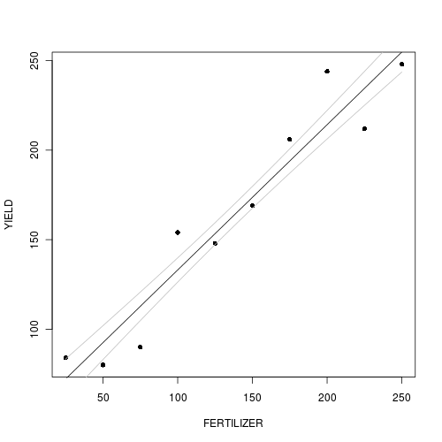
   > vc <- vcov(fert.lm)

   > se <- sqrt(diag(cc %*% vc %*% t(cc)))

   > head(se)

   [1] 11.16695 11.00713 10.84830 10.69048 10.53374 10.37811

5. Reconstruct the summary plot with the derived fit, standard errors and confidence intervals

   > plot(YIELD ~ FERTILIZER, fert, pch = 16)

   > points(newY[1, ] ~ newX, type = "l")

   > points(newY[1, ] - se ~ newX, type = "l", col = "grey")

   > points(newY[1, ] + se ~ newX, type = "l", col = "grey")

   > lwrCI <- newY[1, ] + qnorm(0.025) * se

   > uprCI <- newY[1, ] + qnorm(0.975) * se

   > points(lwrCI ~ newX, type = "l", col = "blue")

   > points(uprCI ~ newX, type = "l", col = "blue")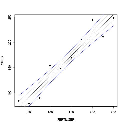

   

Contrasts in linear mixed effects models

For the next demonstration, I will use completely fabricated data. Perhaps one day I will seek out a good example with real data, but for now, the artificial data will do.

Create the artificial data

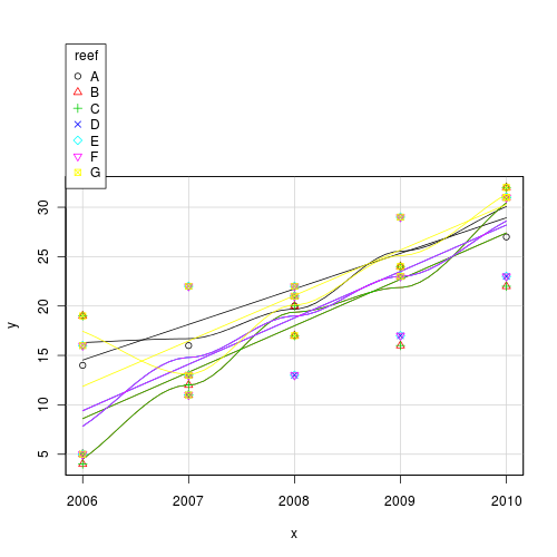
This data set consists of fish counts over time on seven reefs (you can tell it is artificial, because they have increased ;^) Lets fit the generalized linear mixed effects model relating fish counts (y) to year (x). To do so, we will employ the glmmPQL() function from within the MASS package. The glmmPQL fits generalized linear mixed effects models with penalized quasi-likelihood estimation. We will initially use a Gaussian (Normal) error distribution.

Use the predict() function to extract the line of best fit and standard errors

You may well have noticed that although we asked for standard errors of the predictions, we did not receive them. The overloaded predict() function only provides standard errors for simple linear and generalized linear models (not mixed effects models). This is one of the reasons we are exploring the use of contrasts - so that we can derive these things manually.

Use contrasts and matrix algebra to derive predictions and errors

1. First retrieve the fitted model parameters (intercept and slope) for the fixed effects.

   > coefs <- data.lme$coef$fixed

   > coefs

    (Intercept)            x 

   -7875.171429     3.928571 

2. Generate a model matrix appropriate for the predictor variable range. The more numbers there are over the range the smoother (less jagged) the fitted curve.

   > newX <- seq(2006, 2010, l = 100)

   > cc <- as.matrix(expand.grid(1, newX))

   > head(cc)

        Var1     Var2

   [1,]    1 2006.000

   [2,]    1 2006.040

   [3,]    1 2006.081

   [4,]    1 2006.121

   [5,]    1 2006.162

   [6,]    1 2006.202

3. Calculate (derive) the predicted fish counts over time across all reefs.

   > newY <- coefs %*% t(cc)

   > newY

            [,1]     [,2]     [,3]     [,4]     [,5]     [,6]     [,7]     [,8]

   [1,] 5.542857 5.701587 5.860317 6.019048 6.177778 6.336508 6.495238 6.653968

            [,9]    [,10]    [,11]    [,12]    [,13]    [,14]    [,15]   [,16]

   [1,] 6.812698 6.971429 7.130159 7.288889 7.447619 7.606349 7.765079 7.92381

          [,17]   [,18] [,19]   [,20]   [,21]   [,22]    [,23]    [,24]    [,25]

   [1,] 8.08254 8.24127   8.4 8.55873 8.71746 8.87619 9.034921 9.193651 9.352381

           [,26]    [,27]    [,28]    [,29]    [,30]    [,31]    [,32]    [,33]

   [1,] 9.511111 9.669841 9.828571 9.987302 10.14603 10.30476 10.46349 10.62222

           [,34]    [,35]    [,36]    [,37]    [,38]   [,39]    [,40]    [,41]

   [1,] 10.78095 10.93968 11.09841 11.25714 11.41587 11.5746 11.73333 11.89206

           [,42]    [,43]    [,44]    [,45]    [,46]    [,47]    [,48]   [,49]

   [1,] 12.05079 12.20952 12.36825 12.52698 12.68571 12.84444 13.00317 13.1619

           [,50]    [,51]   [,52]    [,53]    [,54]    [,55]    [,56]    [,57]

   [1,] 13.32063 13.47937 13.6381 13.79683 13.95556 14.11429 14.27302 14.43175

           [,58]    [,59]    [,60]    [,61]   [,62]    [,63]    [,64]    [,65]

   [1,] 14.59048 14.74921 14.90794 15.06667 15.2254 15.38413 15.54286 15.70159

           [,66]    [,67]    [,68]    [,69]    [,70]    [,71]   [,72]    [,73]

   [1,] 15.86032 16.01905 16.17778 16.33651 16.49524 16.65397 16.8127 16.97143

           [,74]    [,75]    [,76]    [,77]    [,78]    [,79]    [,80]    [,81]

   [1,] 17.13016 17.28889 17.44762 17.60635 17.76508 17.92381 18.08254 18.24127

        [,82]    [,83]    [,84]    [,85]    [,86]    [,87]    [,88]    [,89]

   [1,]  18.4 18.55873 18.71746 18.87619 19.03492 19.19365 19.35238 19.51111

           [,90]    [,91]   [,92]    [,93]    [,94]    [,95]    [,96]    [,97]

   [1,] 19.66984 19.82857 19.9873 20.14603 20.30476 20.46349 20.62222 20.78095

           [,98]    [,99]   [,100]

   [1,] 20.93968 21.09841 21.25714

4. Calculate (derive) the standard errors of the predicted fish counts.

   > vc <- vcov(data.lme)

   > se <- sqrt(diag(cc %*% vc %*% t(cc)))

   > head(se)

   [1] 0.5931468 0.5911899 0.5892667 0.5873775 0.5855225 0.5837022

5. Make a data frame to hold the predicted values, standard errors and confidence intervals

   > mat <- data.frame(x = newX, fit = newY[1, ], se = se, lwr = newY[1,

   > ] + qnorm(0.025) * se, upr = newY[1, ] + qnorm(0.975) * se)

   > head(mat)

            x      fit        se      lwr      upr

   1 2006.000 5.542857 0.5931468 4.380311 6.705403

   2 2006.040 5.701587 0.5911899 4.542876 6.860298

   3 2006.081 5.860317 0.5892667 4.705376 7.015259

   4 2006.121 6.019048 0.5873775 4.867809 7.170286

   5 2006.162 6.177778 0.5855225 5.030175 7.325381

   6 2006.202 6.336508 0.5837022 5.192473 7.480543

6. Finally, lets plot the data with the predicted trend and confidence intervals overlaid
   > plot(y ~ x, data, pch = as.numeric(data$reef), col = "grey")
   > lines(fit ~ x, mat, col = "black")
   > lines(lwr ~ x, mat, col = "grey")
   > lines(upr ~ x, mat, col = "grey")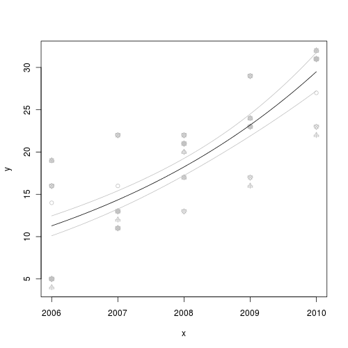

   

Contrasts in generalized linear mixed effects models

The next demonstration, will use very similar data to the previous example, except that a Poisson error distribution would be more appropriate (due to the apparent relationship between mean and variance).

Create the artificial data

This data set consists of fish counts over time on seven reefs (you can tell it is artificial, because they have increased ;^)

Lets fit the generalized linear mixed effects model relating fish counts (y) to year (x). To do so, we will employ the glmmPQL() function from within the MASS package. The glmmPQL fits generalized linear mixed effects models with penalized quasi-likelihood estimation. This time we will use a Poisson distribution distribution.

Use contrasts and matrix algebra to derive predictions and errors

1. First retrieve the fitted model parameters (intercept and slope) for the fixed effects.

   > coefs <- data.lme$coef$fixed

   > coefs <- coefs

   > coefs

    (Intercept)            x 

   -479.5766067    0.2402791 

2. Generate a model matrix appropriate for the predictor variable range. The more numbers there are over the range the smoother (less jagged) the fitted curve.

   > newX <- seq(2006, 2010, l = 100)

   > cc <- as.matrix(expand.grid(1, newX))

   > head(cc)

        Var1     Var2

   [1,]    1 2006.000

   [2,]    1 2006.040

   [3,]    1 2006.081

   [4,]    1 2006.121

   [5,]    1 2006.162

   [6,]    1 2006.202

3. Calculate (derive) the predicted fish counts over time across all reefs. As is, these will be on the log scale, since the canonical link function for a Poisson distribution is a log function. Exponentiation will put this back in scale of the response (fish counts)

   > newY <- exp(coefs %*% t(cc))

   > newY

            [,1]     [,2]     [,3]     [,4]     [,5]     [,6]     [,7]     [,8]

   [1,] 11.28225 11.39231 11.50345 11.61567 11.72899 11.84341 11.95895 12.07561

            [,9]    [,10]    [,11]    [,12]    [,13]   [,14]    [,15]    [,16]

   [1,] 12.19342 12.31237 12.43249 12.55377 12.67624 12.7999 12.92477 13.05086

           [,17]    [,18]    [,19]    [,20]    [,21]    [,22]   [,23]    [,24]

   [1,] 13.17818 13.30674 13.43655 13.56763 13.69999 13.83364 13.9686 14.10487

           [,25]    [,26]    [,27]    [,28]    [,29]    [,30]    [,31]  [,32]

   [1,] 14.24247 14.38141 14.52171 14.66338 14.80643 14.95087 15.09672 15.244

           [,33]    [,34]    [,35]    [,36]    [,37]    [,38]    [,39]    [,40]

   [1,] 15.39271 15.54288 15.69451 15.84761 16.00222 16.15833 16.31596 16.47513

           [,41]    [,42]    [,43]    [,44]    [,45]   [,46]    [,47]    [,48]

   [1,] 16.63585 16.79815 16.96202 17.12749 17.29458 17.4633 17.63366 17.80569

           [,49]    [,50]   [,51]    [,52]    [,53]    [,54]    [,55]   [,56]

   [1,] 17.97939 18.15479 18.3319 18.51074 18.69132 18.87366 19.05778 19.2437

           [,57]  [,58]    [,59]    [,60]    [,61]    [,62]    [,63]    [,64]

   [1,] 19.43144 19.621 19.81241 20.00569 20.20086 20.39793 20.59692 20.79786

           [,65]    [,66]    [,67]    [,68]    [,69]   [,70]    [,71]    [,72]

   [1,] 21.00075 21.20562 21.41249 21.62138 21.83231 22.0453 22.26036 22.47752

          [,73]    [,74]   [,75]    [,76]    [,77]    [,78]    [,79]    [,80]

   [1,] 22.6968 22.91822 23.1418 23.36756 23.59553 23.82571 24.05814 24.29284

           [,81]    [,82]    [,83]    [,84]    [,85]    [,86]    [,87]    [,88]

   [1,] 24.52983 24.76913 25.01077 25.25476 25.50114 25.74991 26.00112 26.25477

          [,89]    [,90]    [,91]    [,92]    [,93]    [,94]    [,95]    [,96]

   [1,] 26.5109 26.76953 27.03068 27.29438 27.56065 27.82952 28.10101 28.37515

           [,97]    [,98]    [,99]   [,100]

   [1,] 28.65196 28.93148 29.21372 29.49872

4. Calculate (derive) the standard errors of the predicted fish counts. Again, these need to be corrected if they are to be on the response scale. This is done by multiplying the standard error estimates by the exponential fitted estimates.

   > vc <- vcov(data.lme)

   > se <- sqrt(diag(cc %*% vc %*% t(cc)))

   > se <- se * newY[1, ]

   > head(se)

   [1] 0.6003354 0.5988101 0.5972302 0.5955962 0.5939090 0.5921693

5. Make a data frame to hold the predicted values, standard errors and confidence intervals

   > mat <- data.frame(x = newX, fit = newY[1, ], se = se, lwr = newY[1,

   > ] + qnorm(0.025) * se, upr = newY[1, ] + qnorm(0.975) * se)

   > head(mat)

            x      fit        se      lwr      upr

   1 2006.000 11.28225 0.6003354 10.10561 12.45888

   2 2006.040 11.39231 0.5988101 10.21866 12.56596

   3 2006.081 11.50345 0.5972302 10.33290 12.67400

   4 2006.121 11.61567 0.5955962 10.44832 12.78302

   5 2006.162 11.72899 0.5939090 10.56495 12.89303

   6 2006.202 11.84341 0.5921693 10.68278 13.00404

6. Finally, lets plot the data with the predicted trend and confidence intervals overlaid
   > plot(y ~ x, data, pch = as.numeric(data$reef), col = "grey")
   > lines(fit ~ x, mat, col = "black")
   > lines(lwr ~ x, mat, col = "grey")
   > lines(upr ~ x, mat, col = "grey")

   

Contrasts in Single Factor ANOVA

Linear model effects parameterization for single factor ANOVA looks like:

yi = μ + βi xi + εi
εi ∼ Normal(0,σ2)	#Residual 'random' effects

Motivating example

Lets say we had measured a response (e.g. weight) from four individuals (replicates) treated in one of three ways (three treatment levels).

Download fish data set

Raw data	Treatment means
FactA: a1 38.12, 40.55, 37.49, 44.79 FactA: a2 50.99, 47.54, 51.46, 52.21 FactA: a3 56.73, 54.08, 59.54, 56.17	FactA: a1 FactA: a2 FactA: a3 Mean 40.24 50.55 56.63

yi = μ + βi xi + εi
y = μ + β1 x1 + β2 x2 + β3 x3 + εi	# over-parameterized model
y = β1 x1 + β2 x2 + β3 x3 + εi	# means parameterization model
y = Intercept + β2 x2 + β3 x3 + εi	# effects parameterization model

Two alternative model parameterizations (based on treatment contrasts) would be:

Means parameterization	Effects parameterization
Data Model parameters Response FactA FactAa1 FactAa2 FactAa3 38.12 a1 1.00 0.00 0.00 40.55 a1 1.00 0.00 0.00 37.49 a1 1.00 0.00 0.00 44.79 a1 1.00 0.00 0.00 50.99 a2 0.00 1.00 0.00 47.54 a2 0.00 1.00 0.00 51.46 a2 0.00 1.00 0.00 52.21 a2 0.00 1.00 0.00 56.73 a3 0.00 0.00 1.00 54.08 a3 0.00 0.00 1.00 59.54 a3 0.00 0.00 1.00 56.17 a3 0.00 0.00 1.00	Data Model parameters Response FactA Intercept FactAa2 FactAa3 38.12 a1 1.00 0.00 0.00 40.55 a1 1.00 0.00 0.00 37.49 a1 1.00 0.00 0.00 44.79 a1 1.00 0.00 0.00 50.99 a2 1.00 1.00 0.00 47.54 a2 1.00 1.00 0.00 51.46 a2 1.00 1.00 0.00 52.21 a2 1.00 1.00 0.00 56.73 a3 1.00 0.00 1.00 54.08 a3 1.00 0.00 1.00 59.54 a3 1.00 0.00 1.00 56.17 a3 1.00 0.00 1.00

Whilst the above two are equivalent for simple designs (such as that illustrated), the means parameterization (that does not include an intercept, or overall mean) is limited to simple single factor designs. Designs that involve additional predictors can only be accommodated via effects parameterization.

Lets now fit the above means and effects parameterized models and contrasts the estimated parameters:

Means parameterization	Effects parameterization
> summary(lm(Response ~ -1 + FactA, fish))$coef         Estimate Std. Error  t value     Pr(>|t|) FactAa1  40.2375   1.300481 30.94046 1.885834e-10 FactAa2  50.5500   1.300481 38.87022 2.453386e-11 FactAa3  56.6300   1.300481 43.54541 8.871078e-12	> summary(lm(Response ~ FactA, fish))$coef             Estimate Std. Error   t value     Pr(>|t|) (Intercept)  40.2375   1.300481 30.940464 1.885834e-10 FactAa2      10.3125   1.839159  5.607184 3.312139e-04 FactAa3      16.3925   1.839159  8.913043 9.243186e-06

The model on the left omits the intercept and thus estimates the treatment means. The parameters estimated by the model on the right are the mean of the first treatment level and the differences between each of the other treatment means and the first treatment mean. If there were only two treatment levels or first treatment was a control (two which you wish to compare the other treatment means), then the effects model is providing what the statisticians are advocating - estimates of the effect sizes as well as estimates of precision (standard error from which confidence intervals can easily be derived).

Derived parameters - simple contrasts

These parameters represent model coefficients that can be substituted back into a linear model. They represent the set of linear constants in the linear model. We can subsequently multiply these parameters to produce alternative linear combinations in order to estimate other values from the linear model.

yi = μ + βi xi

yi = μ + β2 x2 + β2 x2

yi = 40.2375 × a1 + 10.3125 × a2 + 16.3925 × a3

For example, if we wanted to estimate the effect size for the difference between treatments a2 and a3, we could make a1=0, a2=1 and a3=-1. That is, if we multiplied our model parameters by a contrast matrix of 0,1,-1;

The matrix;

a1 a2 a3

is a matrix of contrast coefficients. Each row corresponds to a column in the parameter matrix (vector). The contrast matrix can have multiple columns, each corresponding to a different derived comparison.

yi = 40.2375 × a1 + 10.3125 × a2 + 16.3925 × a3

yi = 40.2375 × 0 + 10.3125 × 1 + 16.3925 × -1

yi = 10.3125 - 16.3925

yi = -6.080

Planned comparisons

Some researchers might be familiar with the use of contrasts in performing so called 'planned comparisons' or 'planned contrasts'. This involves redefining the actual parameters used in the linear model to reflect more meaningful comparisons amongst groups. For example, rather than compare each group mean against the mean of one (the first) treatment group, we many wish to include a comparison of the first treatment group (perhaps a control group) against the average two other treatment groups.

In so doing, this technique provides a relatively easy way to test other non-standard hypotheses (linear effects).

However, a greater understanding of contrasts has even greater benefits when it comes to calculations of effect sizes, marginal means and their associated confidence intervals - features that are considered of greater interpretive value than hypothesis tests. Contrasts can also be used to derive a range of other derived parameters from the fitted model.

Calculating treatment means (and confidence intervals) from the effects model

A simple way to illustrate the use of contrasts to derive new parameters from a linear model is in the estimation of population treatment means from the effects model.

Calculating all the pairwise effects (and confidence intervals) from the effects model

Contrasts in factorial ANOVA

Motivating example

We now extend this example such that each individual fish was subjected to one of five levels of one treatment and one of three levels of another treatment. There were four replicate fish in each treatment combination.

Note, this is an artificial data set. Most of the data sets used in this Workshop series have been real data sets. Real datasets are useful as they provide 'real world' examples of how to apply statistical principles and tools. However, for understanding some techniques, fabricated data allows us to explore techniques under controlled conditions. Furthermore, they allow us to compare statistical outcomes and patterns derived from statistical techniques to the 'truth'. Recall that the purpose of statistics is to 'estimate' population parameters. Fabricating data allows us to know the true values of the parameters that we are trying to estimate and thus allow us to evaluate the accuracy of our outcomes and understanding. I apologise if the use of artificial data causes you any pain or personal hardship.

In the creation of these data, I will be defining the 'true' (theoretical) effect sizes and level of 'noise'.

Download fish1 data set

Simple sample means

We will now calculate the sample means of each FactA by FactB combination. These are called 'cell means' as they are the means of each cell in a table in which the levels of FactA and FactB are the rows and columns (as was depicted in the table above for the theoretical means). If the samples are collected in an unbiased manner (whereby the collected samples reflect the populations), then the cell means should roughly approximate the true means of the underlying populations from whcih the observations were drawn.

Raw sample group means: And the differences between the theoretical means (which DID NOT contain any observational variance) and these raw sample group means:

Here is a side-by-side comparison of the theoretical means, the raw sample means and the cell differences:

Theoretical cell means	Sample cell means	Differences
b1 b2 b3 a1 40.00 45.00 50.00 a2 30.00 33.00 44.00 a3 35.00 43.00 45.00 a4 45.00 50.00 58.00 a5 50.00 59.00 58.00	b1 b2 b3 a1 40.24 45.55 51.63 a2 28.68 34.76 43.84 a3 34.20 43.90 43.91 a4 46.06 50.63 57.80 a5 50.42 60.97 57.27	b1 b2 b3 a1 -0.24 -0.55 -1.63 a2 1.32 -1.76 0.16 a3 0.80 -0.90 1.09 a4 -1.06 -0.63 0.20 a5 -0.42 -1.97 0.73

The sum of the deviations (differences) of the sample means from the theoretical means is:

Modeled population means

Alternatively, we can estimate the cell means based on a full multiplicative linear model.

y_ij = µ + α_i + β_j + αβ_ij

Note that this model is over-parameterized - that is, there are more parameters to estimate than there are groups of data from which to independently estimate them.

The effects parameterization of this model via treatment contrasts incorporates the mean of the first cell (µ) followed by a series of differences. In all, there are 15 groups (five levels of FactA multiplied by three levels of FactB) and correspondingly, there are 15 parameters being estimated:

y_ij = µ + β1 + β2 + β3 + β4 + β5 + β6 + β7 + β8 + β9 + β10 + β11 + β12 + β13 + β14

These parameters correspond to the following:

Model term	Summarized model parameter (name given in R)	Interpretation
µ	(Intercept)	(a1b1)
β1	FactAa2	(a2b1 - a1b1)
β2	FactAa3	(a3b1 - a1b1)
β3	FactAa4	(a4b1 - a1b1)
β4	FactAa5	(a5b1 - a1b1)
β5	FactBb2	(a1b2 - a1b1)
β6	FactBb3	(a1b3 - a1b1)
β7	FactAa2:FactBb2	(a2b1+a1b2) - (a1b1+a2b2)
β8	FactAa3:FactBb2	(a3b1+a1b2) - (a1b1+a3b2)
β9	FactAa4:FactBb2	(a4b1+a1b2) - (a1b1+a4b2)
β10	FactAa5:FactBb2	(a5b1+a1b2) - (a1b1+a5b2)
β11	FactAa2:FactBb3	(a2b1+a1b3) - (a1b1+a2b3)
β12	FactAa3:FactBb3	(a3b1+a1b3) - (a1b1+a3b3)
β13	FactAa4:FactBb3	(a4b1+a1b3) - (a1b1+a4b3)
β14	FactAa5:FactBb3	(a5b1+a1b3) - (a1b1+a5b3)

In R, the linear model is fitted via the lm() function.

Whilst these parameters satisfy the model parameterization, interpretating and utilizing the estimated parameters can take some getting used to. Lets begin by summarizing the estimates of the 15 model parameters.

But this is where the good stuff begins. As the parameters are defined to encapsulate all of the patterns amongst the groups, the linear combination of parameters can now be used to calculate a whole range of related derived estimates (and their standard deviations etc) including:

• population cell means
• marginal means (row and column means)
• effect sizes (differences between marginal means)
• effect sizes (deviations from overall mean)

In order to achieve this wizardry, we must indicate which combination of the parameter estimates are relevant for each of the derived estimates required. And this is where contrast coefficients come in. The contrast coefficients are a set of numbers (equal in length to the number of model parameters) that determine the combinations and weights of the model parameters that are appropriate for each of the derived estimates. Hence when the set of model parameters are multiplied by a single set of contrast coefficients and then summed up, the result is a new derived estimate.

By way of example, the following contrast would specify that the derived estimate should include only (and all of) the first model parameter (and thus according to the table above, estimate the mean of cell FactA level a1 and FactB level b1). In R, the %*% is a special operator that performs matrix multiplication (each element of one matrix is multiplied by the corresponding elements of the other matrix) and returns their sum.

In the above, we indicated that only the first model parameter should be included in deriving the specified estimate, as all the others parameters are multiplied by zeros.

We can calculate multiple derived estimates at once, by multiplying the model parameters by multiple sets of contrast coefficients (represented as a matrix). That is, matrix multiplication. Hence to also calculate the cell mean of FactA level a2 and FactB b1 (a2b1), we would specify the first (a1b1 cell mean) and second (difference between a2b1 and a1b1 cell means) contrasts as ones (1) and the others zeros.

The cbind() function binds together vectors into the columns of a matrix.

At this point we could go on and attempt to work out which combinations of model parameters would be required to define each of the cell means. Whilst it is reasonably straight forward to do this for cells a1b1, a2b1, a3b1, a4b1, a5b1, a1b2, a1b3 (those along the top and down the left column), it requires more mental gymnastics to arrive at the entire set. However, there is a function in R called model.matrix() that helps us achieve this in a relatively pain-free manner. The model.matrix() function gives the design matrix that is used in linear modelling to indicate group membership of categorical variables and in general provides the link between the observed data (response) and the linear combination of predictor variables.

As just eluded to, model.matrix relates each individual observation. However, we are not interested in estimating ('predicting') each observation, we want to predict the means of groups of observations. Hence, we need to reduce the matrix down to the level of the groups.

There are a couple of ways that we could reduce this matrix down to the level of the groups

• As the model contains only categorical predictors, we can just return a unique version (one without duplicates)

  > mat <- unique(model.matrix(fish1.lm))

  > head(mat)

     (Intercept) FactAa2 FactAa3 FactAa4 FactAa5 FactBb2 FactBb3 FactAa2:FactBb2

  1            1       0       0       0       0       0       0               0

  5            1       0       0       0       0       1       0               0

  9            1       0       0       0       0       0       1               0

  13           1       1       0       0       0       0       0               0

  17           1       1       0       0       0       1       0               1

  21           1       1       0       0       0       0       1               0

     FactAa3:FactBb2 FactAa4:FactBb2 FactAa5:FactBb2 FactAa2:FactBb3

  1                0               0               0               0

  5                0               0               0               0

  9                0               0               0               0

  13               0               0               0               0

  17               0               0               0               0

  21               0               0               0               1

     FactAa3:FactBb3 FactAa4:FactBb3 FactAa5:FactBb3

  1                0               0               0

  5                0               0               0

  9                0               0               0

  13               0               0               0

  17               0               0               0

  21               0               0               0

• A more universal technique is to aggregate (summarize) the design matrix according to the factor levels. This technique also allows us to generate contrasts for marginal means and handles models that also include continuous covariates.
  # We take the design matrix converted into a data frame
  # split the design matrix up into subsets according to the levels of FactA and FactB in the fish1 dataframe
  # Apply the mean function to each column of these subsets
  # Combine the means from each subset into a single data frame
  # Retain all but the first two columns (which correspond to the the splitting variables that are appended
  # onto the dataframe)
  # It is then vitally important that the resulting dataframe be converted into a matrix to allow
  # proper matrix multiplications
  

  > library(plyr)

  > mat <- ddply(as.data.frame(model.matrix(fish1.lm)), ~fish1$FactA +

  > fish1$FactB, function(df) mean(df))[, -1:-2]

  > mat <- as.matrix(mat)

  > head(mat)

       (Intercept) FactAa2 FactAa3 FactAa4 FactAa5 FactBb2 FactBb3

  [1,]           1       0       0       0       0       0       0

  [2,]           1       0       0       0       0       1       0

  [3,]           1       0       0       0       0       0       1

  [4,]           1       1       0       0       0       0       0

  [5,]           1       1       0       0       0       1       0

  [6,]           1       1       0       0       0       0       1

       FactAa2:FactBb2 FactAa3:FactBb2 FactAa4:FactBb2 FactAa5:FactBb2

  [1,]               0               0               0               0

  [2,]               0               0               0               0

  [3,]               0               0               0               0

  [4,]               0               0               0               0

  [5,]               1               0               0               0

  [6,]               0               0               0               0

       FactAa2:FactBb3 FactAa3:FactBb3 FactAa4:FactBb3 FactAa5:FactBb3

  [1,]               0               0               0               0

  [2,]               0               0               0               0

  [3,]               0               0               0               0

  [4,]               0               0               0               0

  [5,]               0               0               0               0

  [6,]               1               0               0               0

Hence, the entire contrast matrix for deriving cell mean estimates would be (Note I will display this as transposed to make it more readable and to facilitate correct matrix multiplication).

	a1b1	a1b2	a1b3	a2b1	a2b2	a2b3	a3b1	a3b2	a3b3	a4b1	a4b2	a4b3	a5b1	a5b2	a5b3
µ	1.00	1.00	1.00	1.00	1.00	1.00	1.00	1.00	1.00	1.00	1.00	1.00	1.00	1.00	1.00
β1	0.00	0.00	0.00	1.00	1.00	1.00	0.00	0.00	0.00	0.00	0.00	0.00	0.00	0.00	0.00
β2	0.00	0.00	0.00	0.00	0.00	0.00	1.00	1.00	1.00	0.00	0.00	0.00	0.00	0.00	0.00
β3	0.00	0.00	0.00	0.00	0.00	0.00	0.00	0.00	0.00	1.00	1.00	1.00	0.00	0.00	0.00
β4	0.00	0.00	0.00	0.00	0.00	0.00	0.00	0.00	0.00	0.00	0.00	0.00	1.00	1.00	1.00
β5	0.00	1.00	0.00	0.00	1.00	0.00	0.00	1.00	0.00	0.00	1.00	0.00	0.00	1.00	0.00
β6	0.00	0.00	1.00	0.00	0.00	1.00	0.00	0.00	1.00	0.00	0.00	1.00	0.00	0.00	1.00
β7	0.00	0.00	0.00	0.00	1.00	0.00	0.00	0.00	0.00	0.00	0.00	0.00	0.00	0.00	0.00
β8	0.00	0.00	0.00	0.00	0.00	0.00	0.00	1.00	0.00	0.00	0.00	0.00	0.00	0.00	0.00
β9	0.00	0.00	0.00	0.00	0.00	0.00	0.00	0.00	0.00	0.00	1.00	0.00	0.00	0.00	0.00
β10	0.00	0.00	0.00	0.00	0.00	0.00	0.00	0.00	0.00	0.00	0.00	0.00	0.00	1.00	0.00
β11	0.00	0.00	0.00	0.00	0.00	1.00	0.00	0.00	0.00	0.00	0.00	0.00	0.00	0.00	0.00
β12	0.00	0.00	0.00	0.00	0.00	0.00	0.00	0.00	1.00	0.00	0.00	0.00	0.00	0.00	0.00
β13	0.00	0.00	0.00	0.00	0.00	0.00	0.00	0.00	0.00	0.00	0.00	1.00	0.00	0.00	0.00
β14	0.00	0.00	0.00	0.00	0.00	0.00	0.00	0.00	0.00	0.00	0.00	0.00	0.00	0.00	1.00

The estimated population cell means are thence derived by multiplying the model parameters by this transposed contrast matrix (Note that the design matrix needs to be transposed such that the model parameters for each derived estimate are arranged into columns):

We can make the presentation of these numbers a little more palatable by arranging them in a table (matrix) and labeling the rows and columns.

Here is a side-by-side comparison of the theoretical means, the raw sample means and the cell differences:

Theoretical cell means	Sample cell means	Model derived cell means
b1 b2 b3 a1 40.00 45.00 50.00 a2 30.00 33.00 44.00 a3 35.00 43.00 45.00 a4 45.00 50.00 58.00 a5 50.00 59.00 58.00	b1 b2 b3 a1 40.24 45.55 51.63 a2 28.68 34.76 43.84 a3 34.20 43.90 43.91 a4 46.06 50.63 57.80 a5 50.42 60.97 57.27	b1 b2 b3 a1 40.24 45.55 51.63 a2 28.68 34.76 43.84 a3 34.20 43.90 43.91 a4 46.06 50.63 57.80 a5 50.42 60.97 57.27

Although this might seem like a tedius way to calculate cell means, keep in mind that this is an example of a simple system. The same framework can be applied to more complex designs (such as nested, blocking, repeated measures - mixed effects models) for which simple sample means are unlikely to be as good at estimating true population means as estimates that are informed by all the FactA by Fact B trends across nesting levels. Furthermore, the model basis (and contrast sets) allows us to get estimates of standard deviations, standard errors and confidence intervals around the derived estimates.

Conditions

In order to make use of matrix algebra, the following formatting conditions must be adhered to:

• the contrast matrix MUST be a matrix not a data frame
• Each column of the matrix represents a single separate derived parameter (contrasts are in columns
• There must be exactly the same number of rows as there are parameters in the model

Standard deviations, standard errors and confidence intervals

Multiplying the contrast matrix by the model parameters derives new parameter estimates (as we have just seen). Multiplying the same contrast matrix by the model variance-covariance matrix derives estimates of the associated standard errors (and thus standard errors and confidence intervals). The variance-covariance matrix contains the variances of the estimated model parameters along the diagonals and the covariances between each parameter pair in the off-diagonals.

On a normal distribution, the mean plus or minus one standard deviation comprise approximately 68% of values. 95% of the data is encompassed by the span of data between the mean plus or minus approximately 2 standard deviations. To be more precise, the 95% of the data in a normal distribution span between the mean the following number of standard deviations:

Therefore, confidence intervals can be calculated from standard errors according to the following equation:

95% CI = μ ± 1.96 × SE

Rather than produce the standard errors and confidence intervals in isolation, it is more useful to combine them into a frame along with the derived estimates (cell means in this case).

In the following code snippet, the function outer() multiplies each of the elements of one array with each of the elements of another array. This is called the outer product of the two arrays. In the code below, outer is used to multiply each of the standard error estimates by the upper and lower critical values for a 95% confidence interval from a normal distribution.

There are a number of wrappers that can be used to perform the above sequence of functions. These include:

• predict() - most modelling functions have a predict() method. Unfortunately standard errors (and therefore confidence intervals) are only supplied for simple linear models.
• esticon() - in the doBy package. Given the model (lm, glm, lme) and the contrast matrix, this function will calculate the estimates and their standard errors (confidence intervals)
• popMeans() - also in the doBy package. Hence this is a convenient function for calculating population means (marginal or otherwise) from lm, glm and lme models (only).

As an example...

Note, there is a slight difference between the confidence intervals that we calculated manually and those calculated by the popMeans() function. When we calculated the confidence intervals manually, we defined the 95% confidence intervals from a normal distribution. By contrast, the popMeans function defines the 95% confidence intervals from a t-distribution. For infinite degrees of freedom, the normal and t-distributions are identical. However, for smaller degrees of freedom (sample sizes), the t-distribution is relatively flatter and wider (and arguably a better reflection of the actual distribution). Consequently, the t-distribution might be considered to be more appropriate for models with small sample sizes.

Therefore, confidence intervals based on the t-distribution can be calculated from standard errors according to the following equation:

95% CI = μ ± t0.05,df × SE

where df is the t-distribution's degrees of freedom.

To achieve the same derived confidence intervals manually:

	mu	se	lwr	upr
a1b1	40.24	1.35	37.52	42.96
a1b2	45.55	1.35	42.83	48.27
a1b3	51.63	1.35	48.91	54.35
a2b1	28.68	1.35	25.96	31.40
a2b2	34.76	1.35	32.04	37.48
a2b3	43.84	1.35	41.12	46.56
a3b1	34.20	1.35	31.48	36.92
a3b2	43.90	1.35	41.18	46.62
a3b3	43.91	1.35	41.19	46.63
a4b1	46.06	1.35	43.34	48.78
a4b2	50.63	1.35	47.91	53.35
a4b3	57.80	1.35	55.08	60.52
a5b1	50.42	1.35	47.70	53.14
a5b2	60.97	1.35	58.25	63.69
a5b3	57.27	1.35	54.55	59.99

Interaction plot

If we add columns to this frame that indicate the levels of each of the factors, we can then create an interaction plot that incorporates confidence intervals in addition to the cell mean estimates.

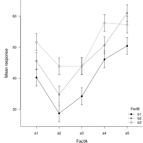
Unfortunately, for more complex designs (particularly those that are hierarchical), identifying or even approximating sensible estimates of degrees of freedom (and thus the t-distributions from which to estimate confidence intervals) becomes increasingly more problematic (and some argue, borders on quess work). As a result, more complex models do not provide any estimates of residual degrees of freedom and thus, it is necessary to either base confidence intervals on the normal distribution or provide your own degrees of freedom (and associated justification). Furthermore, as a result of these complications, the popMeans() function only supports models fitted via lm.

Marginal means

The true flexibility of the contrasts is the ability to derive other estimates, such as the marginal means for the levels of each of the factors. The contrasts for calculating marginal means are the average (averaged over the levels of the specific factor) contrast values for each parameter.

• FactA marginal means
  

  > library(plyr)

  > cmat

  > cmat <- ddply(as.data.frame(model.matrix(fish1.lm)), ~fish1$FactA,

  > function(df) mean(df))

    fish1$FactA (Intercept) FactAa2 FactAa3 FactAa4 FactAa5   FactBb2   FactBb3

  1          a1           1       0       0       0       0 0.3333333 0.3333333

  2          a2           1       1       0       0       0 0.3333333 0.3333333

  3          a3           1       0       1       0       0 0.3333333 0.3333333

  4          a4           1       0       0       1       0 0.3333333 0.3333333

  5          a5           1       0       0       0       1 0.3333333 0.3333333

    FactAa2:FactBb2 FactAa3:FactBb2 FactAa4:FactBb2 FactAa5:FactBb2

  1       0.0000000       0.0000000       0.0000000       0.0000000

  2       0.3333333       0.0000000       0.0000000       0.0000000

  3       0.0000000       0.3333333       0.0000000       0.0000000

  4       0.0000000       0.0000000       0.3333333       0.0000000

  5       0.0000000       0.0000000       0.0000000       0.3333333

    FactAa2:FactBb3 FactAa3:FactBb3 FactAa4:FactBb3 FactAa5:FactBb3

  1       0.0000000       0.0000000       0.0000000       0.0000000

  2       0.3333333       0.0000000       0.0000000       0.0000000

  3       0.0000000       0.3333333       0.0000000       0.0000000

  4       0.0000000       0.0000000       0.3333333       0.0000000

  5       0.0000000       0.0000000       0.0000000       0.3333333

  > class(cmat)

  [1] "data.frame"

  
  # We need to convert this into a matrix and remove the first column (which was only used to help aggregate)
  # We also need to transpose the matrix such that the contrasts are in columns rather than rows

  > cmat <- t(as.matrix(cmat[, -1]))

  
  # Use this contrast matrix to derive new parameters and their standard errors

  > FactAs <- fish1.lm$coef %*% cmat

  > se <- sqrt(diag(t(cmat) %*% vcov(fish1.lm) %*% cmat))

  > ci <- as.numeric(FactAs) + outer(se, qt(df = fish1.lm$df, c(0.025,

  > 0.975)))

  > colnames(ci) <- c("lwr", "upr")

  > mat2 <- cbind(mu = as.numeric(FactAs), se, ci)

  > rownames(mat2) <- levels(fish1$FactA)

  Contrast matrix		Marginal means
  1 2 3 4 5 (Intercept) 1.00 1.00 1.00 1.00 1.00 FactAa2 0.00 1.00 0.00 0.00 0.00 FactAa3 0.00 0.00 1.00 0.00 0.00 FactAa4 0.00 0.00 0.00 1.00 0.00 FactAa5 0.00 0.00 0.00 0.00 1.00 FactBb2 0.33 0.33 0.33 0.33 0.33 FactBb3 0.33 0.33 0.33 0.33 0.33 FactAa2:FactBb2 0.00 0.33 0.00 0.00 0.00 FactAa3:FactBb2 0.00 0.00 0.33 0.00 0.00 FactAa4:FactBb2 0.00 0.00 0.00 0.33 0.00 FactAa5:FactBb2 0.00 0.00 0.00 0.00 0.33 FactAa2:FactBb3 0.00 0.33 0.00 0.00 0.00 FactAa3:FactBb3 0.00 0.00 0.33 0.00 0.00 FactAa4:FactBb3 0.00 0.00 0.00 0.33 0.00 FactAa5:FactBb3 0.00 0.00 0.00 0.00 0.33		mu se lwr upr a1 45.81 0.78 44.24 47.38 a2 35.76 0.78 34.19 37.33 a3 40.67 0.78 39.10 42.24 a4 51.50 0.78 49.93 53.07 a5 56.22 0.78 54.65 57.79

• FactB marginal means
  

  > cmat <- ddply(as.data.frame(model.matrix(fish1.lm)), ~fish1$FactB,

  > function(df) mean(df))

  > cmat <- as.matrix(cmat[, -1])

  > FactBs <- fish1.lm$coef %*% t(cmat)

  > se <- sqrt(diag(cmat %*% vcov(fish1.lm) %*% t(cmat)))

  > ci <- as.numeric(FactBs) + outer(se, qt(df = fish1.lm$df, c(0.025,

  > 0.975)))

  > colnames(ci) <- c("lwr", "upr")

  > mat2 <- cbind(mu = as.numeric(FactBs), se, ci)

  > rownames(mat2) <- levels(fish1$FactB)

  Contrast matrix		Marginal means
  1 2 3 (Intercept) 1.00 1.00 1.00 FactAa2 0.20 0.20 0.20 FactAa3 0.20 0.20 0.20 FactAa4 0.20 0.20 0.20 FactAa5 0.20 0.20 0.20 FactBb2 0.00 1.00 0.00 FactBb3 0.00 0.00 1.00 FactAa2:FactBb2 0.00 0.20 0.00 FactAa3:FactBb2 0.00 0.20 0.00 FactAa4:FactBb2 0.00 0.20 0.00 FactAa5:FactBb2 0.00 0.20 0.00 FactAa2:FactBb3 0.00 0.00 0.20 FactAa3:FactBb3 0.00 0.00 0.20 FactAa4:FactBb3 0.00 0.00 0.20 FactAa5:FactBb3 0.00 0.00 0.20		mu se lwr upr b1 39.92 0.60 38.70 41.14 b2 47.16 0.60 45.94 48.38 b3 50.89 0.60 49.67 52.11

• FactA by FactB interaction marginal means (NOTE, as there are only two factors, this gives the marginal means of the highest order interaction - ie, the cell means)
  

  > cmat <- ddply(as.data.frame(model.matrix(fish1.lm)), ~fish1$FactA +

  > fish1$FactB, function(df) mean(df))

  > cmat <- as.matrix(cmat[, -1:-2])

  > FactAFactBs <- fish1.lm$coef %*% t(cmat)

  > se <- sqrt(diag(cmat %*% vcov(fish1.lm) %*% t(cmat)))

  > se <- sqrt(diag(cmat %*% vcov(fish1.lm) %*% t(cmat)))

  > ci <- as.numeric(FactAFactBs) + outer(se, qt(df = fish1.lm$df,

  > c(0.025, 0.975)))

  > colnames(ci) <- c("lwr", "upr")

  > mat2 <- cbind(mu = as.numeric(FactAFactBs), se, ci)

  > rownames(mat2) <- interaction(with(fish1, expand.grid(levels(FactB),

  > levels(FactA))[, c(2, 1)]), sep = "")

  Contrast matrix
  1 2 3 4 5 6 7 8 9 10 11 12 13 14 15 (Intercept) 1.00 1.00 1.00 1.00 1.00 1.00 1.00 1.00 1.00 1.00 1.00 1.00 1.00 1.00 1.00 FactAa2 0.00 0.00 0.00 1.00 1.00 1.00 0.00 0.00 0.00 0.00 0.00 0.00 0.00 0.00 0.00 FactAa3 0.00 0.00 0.00 0.00 0.00 0.00 1.00 1.00 1.00 0.00 0.00 0.00 0.00 0.00 0.00 FactAa4 0.00 0.00 0.00 0.00 0.00 0.00 0.00 0.00 0.00 1.00 1.00 1.00 0.00 0.00 0.00 FactAa5 0.00 0.00 0.00 0.00 0.00 0.00 0.00 0.00 0.00 0.00 0.00 0.00 1.00 1.00 1.00 FactBb2 0.00 1.00 0.00 0.00 1.00 0.00 0.00 1.00 0.00 0.00 1.00 0.00 0.00 1.00 0.00 FactBb3 0.00 0.00 1.00 0.00 0.00 1.00 0.00 0.00 1.00 0.00 0.00 1.00 0.00 0.00 1.00 FactAa2:FactBb2 0.00 0.00 0.00 0.00 1.00 0.00 0.00 0.00 0.00 0.00 0.00 0.00 0.00 0.00 0.00 FactAa3:FactBb2 0.00 0.00 0.00 0.00 0.00 0.00 0.00 1.00 0.00 0.00 0.00 0.00 0.00 0.00 0.00 FactAa4:FactBb2 0.00 0.00 0.00 0.00 0.00 0.00 0.00 0.00 0.00 0.00 1.00 0.00 0.00 0.00 0.00 FactAa5:FactBb2 0.00 0.00 0.00 0.00 0.00 0.00 0.00 0.00 0.00 0.00 0.00 0.00 0.00 1.00 0.00 FactAa2:FactBb3 0.00 0.00 0.00 0.00 0.00 1.00 0.00 0.00 0.00 0.00 0.00 0.00 0.00 0.00 0.00 FactAa3:FactBb3 0.00 0.00 0.00 0.00 0.00 0.00 0.00 0.00 1.00 0.00 0.00 0.00 0.00 0.00 0.00 FactAa4:FactBb3 0.00 0.00 0.00 0.00 0.00 0.00 0.00 0.00 0.00 0.00 0.00 1.00 0.00 0.00 0.00 FactAa5:FactBb3 0.00 0.00 0.00 0.00 0.00 0.00 0.00 0.00 0.00 0.00 0.00 0.00 0.00 0.00 1.00
  Marginal means
  mu se lwr upr a1b1 40.24 1.35 37.52 42.96 a1b2 45.55 1.35 42.83 48.27 a1b3 51.63 1.35 48.91 54.35 a2b1 28.68 1.35 25.96 31.40 a2b2 34.76 1.35 32.04 37.48 a2b3 43.84 1.35 41.12 46.56 a3b1 34.20 1.35 31.48 36.92 a3b2 43.90 1.35 41.18 46.62 a3b3 43.91 1.35 41.19 46.63 a4b1 46.06 1.35 43.34 48.78 a4b2 50.63 1.35 47.91 53.35 a4b3 57.80 1.35 55.08 60.52 a5b1 50.42 1.35 47.70 53.14 a5b2 60.97 1.35 58.25 63.69 a5b3 57.27 1.35 54.55 59.99

Again, for simple models, it is possible to use the popMeans function to get these marginal means:

Not surprisingly, for simple designs (like simple linear models), multiple bright members of the R community have written functions that derive the marginal means as well as the standard errors of the marginal mean effect sizes. This function is called model.tables().

> model.tables(aov(fish1.lm), type = "means", se = T)

Effect sizes - differences between means

To derive effect sizes, you simply subtract one contrast set from another and use the result as the contrast for the derived parameter.

Effect sizes - for simple main effects

For example, to derive the effect size (difference between two parameters) of a1 vs a2 for the b1 level of Factor B:

THE NAMES IN THE CONTRAST MATRIX ARE NOT CORRECT

Contrast matrix for cell		Contrast matrix for		Effect size for
means (a1b1 & a2b1)		a1b1 - a2b1		a1b1 - a2b1
1 2 (Intercept) 1.00 1.00 FactAa2 0.00 1.00 FactAa3 0.00 0.00 FactAa4 0.00 0.00 FactAa5 0.00 0.00 FactBb2 0.00 0.00 FactBb3 0.00 0.00 FactAa2:FactBb2 0.00 0.00 FactAa3:FactBb2 0.00 0.00 FactAa4:FactBb2 0.00 0.00 FactAa5:FactBb2 0.00 0.00 FactAa2:FactBb3 0.00 0.00 FactAa3:FactBb3 0.00 0.00 FactAa4:FactBb3 0.00 0.00 FactAa5:FactBb3 0.00 0.00	minus	A (Intercept) 0.00 FactAa2 -1.00 FactAa3 0.00 FactAa4 0.00 FactAa5 0.00 FactBb2 0.00 FactBb3 0.00 FactAa2:FactBb2 0.00 FactAa3:FactBb2 0.00 FactAa4:FactBb2 0.00 FactAa5:FactBb2 0.00 FactAa2:FactBb3 0.00 FactAa3:FactBb3 0.00 FactAa4:FactBb3 0.00 FactAa5:FactBb3 0.00	equals	mu se lwr upr 1 11.55 1.91 7.71 15.40

Whilst it is possible to go through and calculate all the rest of the effects individually, we can loop through and create a matrix that contains all the appropriate contrasts.

Effect sizes - for marginal effects (no interactions)

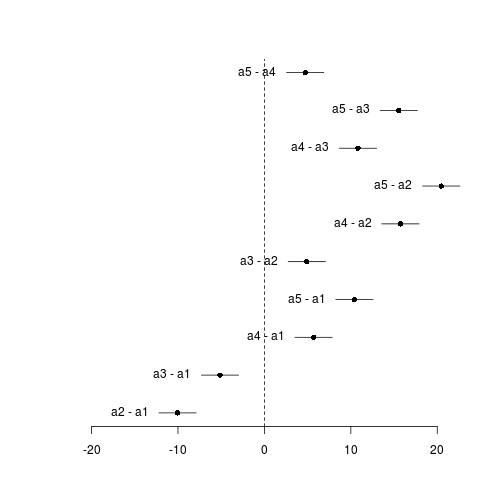
Effect sizes of FactA marginal means

Contrast matrix
a2 - a1 a3 - a1 a4 - a1 a5 - a1 a3 - a2 a4 - a2 a5 - a2 a4 - a3 a5 - a3 a5 - a4 (Intercept) 0.00 0.00 0.00 0.00 0.00 0.00 0.00 0.00 0.00 0.00 FactAa2 1.00 0.00 0.00 0.00 -1.00 -1.00 -1.00 0.00 0.00 0.00 FactAa3 0.00 1.00 0.00 0.00 1.00 0.00 0.00 -1.00 -1.00 0.00 FactAa4 0.00 0.00 1.00 0.00 0.00 1.00 0.00 1.00 0.00 -1.00 FactAa5 0.00 0.00 0.00 1.00 0.00 0.00 1.00 0.00 1.00 1.00 FactBb2 0.00 0.00 0.00 0.00 0.00 0.00 0.00 0.00 0.00 0.00 FactBb3 0.00 0.00 0.00 0.00 0.00 0.00 0.00 0.00 0.00 0.00 FactAa2:FactBb2 0.33 0.00 0.00 0.00 -0.33 -0.33 -0.33 0.00 0.00 0.00 FactAa3:FactBb2 0.00 0.33 0.00 0.00 0.33 0.00 0.00 -0.33 -0.33 0.00 FactAa4:FactBb2 0.00 0.00 0.33 0.00 0.00 0.33 0.00 0.33 0.00 -0.33 FactAa5:FactBb2 0.00 0.00 0.00 0.33 0.00 0.00 0.33 0.00 0.33 0.33 FactAa2:FactBb3 0.33 0.00 0.00 0.00 -0.33 -0.33 -0.33 0.00 0.00 0.00 FactAa3:FactBb3 0.00 0.33 0.00 0.00 0.33 0.00 0.00 -0.33 -0.33 0.00 FactAa4:FactBb3 0.00 0.00 0.33 0.00 0.00 0.33 0.00 0.33 0.00 -0.33 FactAa5:FactBb3 0.00 0.00 0.00 0.33 0.00 0.00 0.33 0.00 0.33 0.33
Marginal means
mu se lwr upr a2 - a1 -10.05 1.10 -12.21 -7.89 a3 - a1 -5.14 1.10 -7.30 -2.98 a4 - a1 5.69 1.10 3.53 7.85 a5 - a1 10.41 1.10 8.25 12.57 a3 - a2 4.91 1.10 2.75 7.07 a4 - a2 15.74 1.10 13.58 17.90 a5 - a2 20.46 1.10 18.30 22.62 a4 - a3 10.83 1.10 8.67 12.99 a5 - a3 15.55 1.10 13.39 17.71 a5 - a4 4.72 1.10 2.56 6.88

Effect sizes plot

> plot(seq(-22, 22, l = nrow(mat2)), 1:nrow(mat2), type = "n",

> ann = F, axes = F)

> abline(v = 0, lty = 2)

> segments(mat2[, "lwr"], 1:nrow(mat2), mat2[, "upr"], 1:nrow(mat2))

> points(mat2[, "mu"], 1:nrow(mat2), pch = 16)

> text(mat2[, "lwr"], 1:nrow(mat2), lab = rownames(mat2), pos = 2)

> axis(1)

Effect sizes of FactB marginal means

Contrast matrix
b2 - b1 b3 - b1 b3 - b2 (Intercept) 0.00 0.00 0.00 FactAa2 0.00 0.00 0.00 FactAa3 0.00 0.00 0.00 FactAa4 0.00 0.00 0.00 FactAa5 0.00 0.00 0.00 FactBb2 1.00 0.00 -1.00 FactBb3 0.00 1.00 1.00 FactAa2:FactBb2 0.20 0.00 -0.20 FactAa3:FactBb2 0.20 0.00 -0.20 FactAa4:FactBb2 0.20 0.00 -0.20 FactAa5:FactBb2 0.20 0.00 -0.20 FactAa2:FactBb3 0.00 0.20 0.20 FactAa3:FactBb3 0.00 0.20 0.20 FactAa4:FactBb3 0.00 0.20 0.20 FactAa5:FactBb3 0.00 0.20 0.20
Marginal means
mu se lwr upr b2 - b1 7.24 0.85 5.57 8.91 b3 - b1 10.97 0.85 9.30 12.64 b3 - b2 3.73 0.85 2.06 5.40

Simple main effects - effects associated with one factor at specific levels of another factor

But what do we do in the presence of an interaction then - when effect sizes of marginal means will clearly be underrepresenting the patterns. The presence of an interaction implies that the effect sizes differ according to the combinations of the factor levels.

For example, lets explore the effects of b1 vs b3 at each of the levels of Factor A

> fits <- NULL

> for (fA in levels(fish1$FactA)) {

> mat <- model.matrix(~FactA * FactB, fish1[fish1$FactA ==

> fA & fish1$FactB %in% c("b1", "b3"), ])

> mat <- unique(mat)

> dat <- fish1[fish1$FactA == fA & fish1$FactB %in% c("b1",

> "b3"), ]

> dat$FactB <- factor(dat$FactB)

> cm <- NULL

> for (i in 1:(nrow(mat) - 1)) {

> for (j in (i + 1):nrow(mat)) {

> nm <- with(dat, paste(levels(FactB)[j], "-", levels(FactB)[i]))

> eval(parse(text = paste("cm <- cbind(cm,'", nm, "'=c(mat[j,]-mat[i,]))")))

> }

> }

> es <- fish1.lm$coef %*% cm

> se <- sqrt(diag(t(cm) %*% vcov(fish1.lm) %*% cm))

> ci <- as.numeric(es) + outer(se, qnorm(c(0.025, 0.975)))

> mat2 <- cbind(mu = as.numeric(es), se, ci)

> fits <- rbind(fits, mat2)

> }

> colnames(fits) <- c("ES", "se", "lwr", "upr")

> rname <- rownames(fits)

> fits <- data.frame(fits)

> fits$FactA <- levels(fish1$FactA)

> fits$Comp <- factor(rname)

> fits

ES se lwr upr FactA Comp 1 11.4 1.9 7.6 15 a1 b3 - b1 2 15.2 1.9 11.4 19 a2 b3 - b1 3 9.7 1.9 6.0 13 a3 b3 - b1 4 11.7 1.9 8.0 15 a4 b3 - b1 5 6.9 1.9 3.1 11 a5 b3 - b1

Compare each level of FactB at each level of FactA

> oo <- outer(FactAs, FactBs, FUN = "+")/2

> dat <- fish1[fish1$FactA %in% levels(fish1$FactA) & fish1$FactB ==

> "b1", ]

> mat <- unique(model.matrix(~FactA * FactB, fish1 = dat))

> fish1.lm$coef %*% t(mat)

1 5 9 13 17 21 25 29 33 37 41 45 49 53 57 40 46 52 29 35 44 34 44 44 46 51 58 50 61 57

> model.tables(aov(fish1.lm), type = "means", se = T)

-->

Welcome to the end of this tutorial