Workshop 3 - simple regression
23 April 2011
Basic statistics references
- Logan (2010) - Chpt 8
- Quinn & Keough (2002) - Chpt 5
Simple linear regression
Here is an example from Fowler, Cohen and Parvis (1998). An agriculturalist was interested in the effects of fertilizer load on the yield of grass. Grass seed was sown uniformly over an area and different quantities of commercial fertilizer were applied to each of ten 1 m2 randomly located plots. Two months later the grass from each plot was harvested, dried and weighed. The data are in the file fertilizer.csv.
Download Fertilizer data set
| Format of fertilizer.csv data files | |||||||||||||||||||
|---|---|---|---|---|---|---|---|---|---|---|---|---|---|---|---|---|---|---|---|
|
 |
||||||||||||||||||
Show code
- The biological hypothesis of interest
- The biological null hypothesis of interest
- The statistical null hypothesis of interest

- sample y-intercept
- sample slope
- t value for main H0
- R2 value
Simple linear regression
Christensen et al. (1996) studied the relationships between coarse woody debris (CWD) and, shoreline vegetation and lake development in a sample of 16 lakes. They defined CWD as debris greater than 5cm in diameter and recorded, for a number of plots on each lake, the basal area (m2.km-1) of CWD in the nearshore water, and the density (no.km-1) of riparian trees along the shore. The data are in the file christ.csv and the relevant variables are the response variable, CWDBASAL (coarse woody debris basal area, m2.km-1), and the predictor variable, RIPDENS (riparian tree density, trees.km-1).
Download Christensen data set
| Format of christ.csv data files | ||||||||||||||||||||||||||||
|---|---|---|---|---|---|---|---|---|---|---|---|---|---|---|---|---|---|---|---|---|---|---|---|---|---|---|---|---|
|
 |
|||||||||||||||||||||||||||
- The biological hypothesis of interest
- The biological null hypothesis of interest
- The statistical null hypothesis of interest
| Assumption | Diagnostic/Risk Minimization |
|---|---|
| I. | |
| II. | |
| III. | |
| IV. |

- Is there any evidence of nonlinearity? (Y or N)
- Is there any evidence of nonnormality? (Y or N)
- Is there any evidence of unequal variance? (Y or N)

- sample y-intercept
- sample slope
- t value for main H0
- P-value for main H0
- R2 value
Simple linear regression
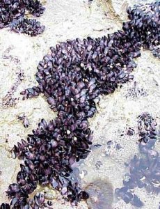
Here is a modified example from Quinn and Keough (2002). Peake & Quinn (1993) investigated the relationship between the number of individuals of invertebrates living in amongst clumps of mussels on a rocky intertidal shore and the area of those mussel clumps.
Download PeakeQuinn data set
| Format of peakquinn.csv data files | |||||||||||||||||||
|---|---|---|---|---|---|---|---|---|---|---|---|---|---|---|---|---|---|---|---|
|
 |
||||||||||||||||||
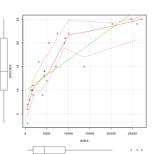
Before performing the analysis we need to check the assumptions. To evaluate the assumptions of linearity, normality and homogeneity of variance, construct a scatterplot of INDIV against AREA (INDIV on y-axis, AREA on x-axis) including a lowess smoother and boxplots on the axes.
- In this case, the researchers are interested in investigating whether there is a relationship between the number of invertebrate individuals and mussel clump area as well as generating a predictive model. However, they are not interested in the specific magnitude of the relationship (slope) and have no intension of comparing their slope to any other non-zero values. Is
model I or II regression
appropriate in these circumstances?. Explain?
- Is there any evidence that the other assumptions are likely to be violated?


- Test the null hypothesis that the population slope of the regression line between log number of individuals and log clump area is zero - use either the t-test or ANOVA F-test regression output. What are your conclusions (statistical and biological)? HINT
- If the relationship is significant construct the regression equation relating the number of individuals in the a clump to the clump size. Remember that parameter estimates should be based on RMA regression not OLS!
DV = intercept + slope x IV Log10Individuals Log10Area
A linear regression of log number of individuals against log clump area showed (choose correct option)
- b (slope):
- c (y-intercept):

Model II RMA regression
Nagy, Girard & Brown (1999) investigated the allometric scaling relationships for mammals (79 species), reptiles (55 species) and birds (95 species). The observed relationships between body size and metabolic rates of organisms have attracted a great deal of discussion amongst scientists from a wide range of disciplines recently. Whilst some have sort to explore explanations for the apparently 'universal' patterns, Nagy et al. (1999) were interested in determining whether scaling relationships differed between taxonomic, dietary and habitat groupings.
Download Nagy data set
| Format of nagy.csv data file | ||||||||||||||||||||||||||||||||||||||||||||||||||||||||
|---|---|---|---|---|---|---|---|---|---|---|---|---|---|---|---|---|---|---|---|---|---|---|---|---|---|---|---|---|---|---|---|---|---|---|---|---|---|---|---|---|---|---|---|---|---|---|---|---|---|---|---|---|---|---|---|---|
|
For this example, we will explore the relationships between field metabolic rate (FMR) and body mass (Mass) in grams for the entire data set and then separately for each of the three classes (mammals, reptiles and aves).
Unlike the previous examples in which both predictor and response variables could be considered 'random' (measured not set), parameter estimates should be based on model II RMA regression. However, unlike previous examples, in this example, the primary focus is not hypothesis testing about whether there is a relationship or not. Nor is prediction a consideration. Instead, the researchers are interested in establishing (and comparing) the allometric scaling factors (slopes) of the metabolic rate - body mass relationships. Hence in this case, model II regression is indeed appropriate.

- Is there any evidence of non-normality?
- Is there any evidence of non-linearity?

Indicate the following;
| OLS | RMA | Class | Slope | Intercept | Slope | Intercept | R2 |
|---|---|---|---|---|---|
| Mammals (HINT and HINT) | |||||
| Reptiles (HINT and HINT) | |||||
| Aves (HINT and HINT) | |||||
- Fit the OLS regression line to this plot (HINT)
- Fit the RMA regression line (in red) to this plot (HINT)

- Complete the following table
OLS RMA Class Slope Intercept Slope Intercept R2 Entire data set (HINT and HINT) - Produce a scatterplot that depicts the relationship between FMR and Mass for the entire data set (HINT)
- Fit the OLS regression line to this plot (HINT)
- Fit the RMA regression line (in red) to this plot (HINT)
- Compare and contrast the OLS and RMA parameter estimates. Explain which estimates are most appropriate and why the in this case the two methods produce not so similar estimates.
