Workshop 4 - multiple and non-linear regression
22 May 2011
Basic statistics references
- Logan (2010) - Chpt 9
- Quinn & Keough (2002) - Chpt 6
Multiple Linear Regression
Paruelo & Lauenroth (1996) analyzed the geographic distribution and the effects of climate variables on the relative abundance of a number of plant functional types (PFT's) including shrubs, forbs, succulents (e.g. cacti), C3 grasses and C4 grasses. They used data from 73 sites across temperate central North America (see pareulo.syd) and calculated the relative abundance of C3 grasses at each site as a response variable
Download Paruelo data set
| Format of paruelo.csv data file | |||||||||||||||||||||||||||
|---|---|---|---|---|---|---|---|---|---|---|---|---|---|---|---|---|---|---|---|---|---|---|---|---|---|---|---|
|
 |
| Assumption | Diagnostic/Risk Minimization |
|---|---|
| I. | |
| II. | |
| III. | |
| IV. | |
| V. |
- Focussing on the assumptions of Normality, Homogeneity of Variance and Linearity, is there evidence of violations of these assumptions (y or n)?
- Try applying a temporary square root transformation (HINT). Does this improve some of these specific assumptions (y or n)?
Show code
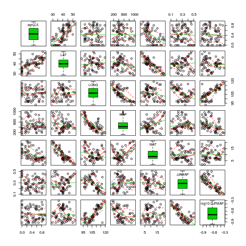
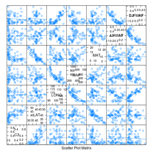
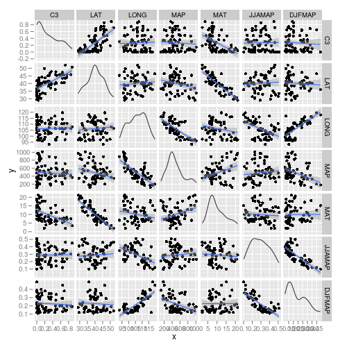
> library(car) > scatterplotMatrix(~sqrt(C3) + LAT + LONG + MAP + MAT + JJAMAP + > log10(DJFMAP), data = paruelo, diagonal = "boxplot") - Is there any evidence that the assumption of Collinearity is likely to be violated (y or n)?
- (Multi)collinearity
occurs when one or more of the predictor variables are correlated to the other predictor variables, therefore this assumption can also be examined by calculating the pairwise correlation coefficients between all the predictor variables (HINT). Which predictor variables are highly correlated?
Show code
> cor(paruelo[, -1]) LAT LONG MAP MAT JJAMAP DJFMAPLAT 1.00000000 0.09655281 -0.2465058 -0.838590413 0.07417497 -0.065124848LONG 0.09655281 1.00000000 -0.7336870 -0.213109100 -0.49155774 0.770743994MAP -0.24650582 -0.73368703 1.0000000 0.355090766 0.11225905 -0.404512409MAT -0.83859041 -0.21310910 0.3550908 1.000000000 -0.08077131 0.001478037JJAMAP 0.07417497 -0.49155774 0.1122590 -0.080771307 1.00000000 -0.791540381DJFMAP -0.06512485 0.77074399 -0.4045124 0.001478037 -0.79154038 1.000000000
- Calculate the VIF values for each of the predictor variables (HINT).
- Calculate the tolerance values for each of the predictor variables (HINT).
Show code> library(car) > vif(lm(sqrt(paruelo$C3) ~ LAT + LONG + MAP + MAT + JJAMAP + log10(DJFMAP), > data = paruelo)) LAT LONG MAP MAT JJAMAP3.560103 4.988318 2.794157 3.752353 3.194724log10(DJFMAP)5.467330> library(car) > 1/vif(lm(sqrt(paruelo$C3) ~ LAT + LONG + MAP + MAT + JJAMAP + > log10(DJFMAP), data = paruelo)) LAT LONG MAP MAT JJAMAP0.2808908 0.2004684 0.3578897 0.2664995 0.3130161log10(DJFMAP)0.1829046Predictor VIF Tolerance LAT LONG MAP MAT JJAMAP log10(DJFMAP) - Is there any evidence of (multi)collinearity, and if so, which variables are responsible for violations of this assumption?
We obviously cannot easily incorporate all 6 predictors into the one model, because of the collinearity problem. Paruelo and Lauenroth (1996) separated the predictors into two groups for their analyses. One group included LAT and LONG and the other included MAP, MAT, JJAMAP and DJFMAP. We will focus on the relationship between the square root relative abundance of C3 plants and latitude and longitude. This relationship will investigate the geographic pattern in abundance of C3 plants.
- Write out the full multiplicative model
- Check the assumptions of this linear model. In particular, check collinearity. HINT
Show code
> library(car) > scatterplotMatrix(~sqrt(C3) + LAT + LONG, data = paruelo, diagonal = "boxplot") 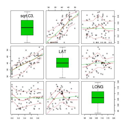
> vif(lm(sqrt(C3) ~ LAT + LONG, data = paruelo)) LAT LONG1.00941 1.00941 - Obviously, this model will violate collinearity. It is highly likely that LAT and LONG will be related to the LAT:LONG interaction term. It turns out that if we center the variables, then the individual terms will no longer be correlated to the interaction. Center the LAT and LONG variables (
HINT) and
(HINT)
Show code
> paruelo$cLAT <- scale(paruelo$LAT, scale = F) > paruelo$cLONG <- scale(paruelo$LONG, scale = F)
- Examine the diagnostic plots (HINT) specially the residual plot to confirm no further evidence of violations of the analysis assumptions
Show code
> paruelo.lm <- lm(sqrt(C3) ~ cLAT * cLONG, data = paruelo) > par(mfrow = c(2, 3), oma = c(0, 0, 2, 0)) > plot(paruelo.lm, ask = F, which = 1:6) 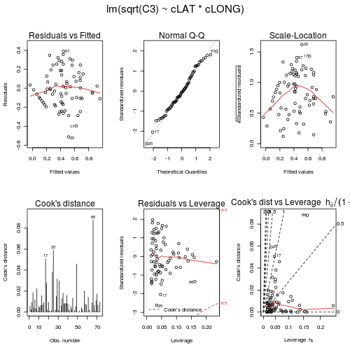
> influence.measures(paruelo.lm) Influence measures oflm(formula = sqrt(C3) ~ cLAT * cLONG, data = paruelo) :dfb.1_ dfb.cLAT dfb.cLON dfb.cLAT. dffit cov.r cook.d hat inf1 -0.02402 -0.083059 -0.084079 -0.121467 -0.15232 1.379 5.88e-03 0.2347 *2 -0.02221 -0.064489 -0.040666 -0.073805 -0.09560 1.227 2.32e-03 0.1389 *3 0.08130 0.134833 0.066766 0.117108 0.18920 1.083 9.00e-03 0.05564 0.18842 0.102837 -0.149242 -0.074613 0.27640 0.957 1.87e-02 0.03175 -0.06669 -0.070090 0.046655 0.023640 -0.11683 1.091 3.45e-03 0.04486 -0.14663 0.020076 0.158421 0.006884 -0.21885 1.001 1.19e-02 0.03057 -0.06266 0.095315 -0.006186 0.047476 -0.11206 1.102 3.17e-03 0.05108 -0.14641 0.034868 0.221772 -0.071379 -0.30117 1.016 2.25e-02 0.05209 -0.03667 0.026450 0.024624 -0.005908 -0.05703 1.088 8.24e-04 0.031710 -0.14355 -0.014721 0.043712 0.016311 -0.15090 0.989 5.65e-03 0.015311 -0.06802 -0.077774 0.052091 0.030960 -0.12872 1.101 4.19e-03 0.053412 -0.09834 0.126501 0.005986 0.046997 -0.15816 1.064 6.29e-03 0.038813 0.11115 -0.093743 -0.111372 0.092157 0.24977 1.061 1.56e-02 0.058014 0.08474 0.046585 -0.103485 -0.077405 0.16432 1.104 6.81e-03 0.062215 -0.10466 0.005614 0.159085 0.003719 -0.19200 1.063 9.25e-03 0.046016 0.02997 0.006031 -0.022676 -0.007923 0.03832 1.082 3.72e-04 0.023417 -0.22231 -0.242042 -0.256005 -0.259471 -0.46135 0.867 5.07e-02 0.046418 -0.15718 -0.195191 -0.167613 -0.197664 -0.33555 0.980 2.77e-02 0.048319 -0.03827 0.067695 0.013203 -0.004632 -0.08826 1.133 1.97e-03 0.070320 0.14881 0.082543 -0.079749 -0.027279 0.19334 0.993 9.27e-03 0.023821 0.02694 -0.052154 0.013621 -0.042509 0.06315 1.184 1.01e-03 0.1064 *22 0.01333 0.036162 0.002225 0.019532 0.03980 1.165 4.02e-04 0.091123 0.03874 -0.041008 -0.026165 0.016163 0.07567 1.106 1.45e-03 0.047524 0.18953 -0.068780 -0.263543 0.120259 0.39649 0.949 3.83e-02 0.052225 -0.30655 -0.141051 -0.348442 -0.174237 -0.50904 0.721 5.92e-02 0.0333 *26 -0.01163 0.020739 -0.004288 0.014771 -0.02450 1.151 1.52e-04 0.079727 -0.06640 -0.035776 0.047618 0.021757 -0.09331 1.073 2.20e-03 0.028728 0.15820 -0.100195 0.156872 -0.087023 0.24687 1.004 1.51e-02 0.037129 0.23271 -0.199428 0.178733 -0.171942 0.36130 0.913 3.16e-02 0.038330 -0.05886 -0.051722 0.023280 0.001329 -0.08413 1.075 1.79e-03 0.027831 0.18206 -0.039000 0.294547 -0.009475 0.34876 0.977 2.98e-02 0.050332 0.04158 0.010092 0.004277 0.002215 0.04358 1.068 4.81e-04 0.014733 -0.11614 0.057069 -0.084317 0.045564 -0.15421 1.033 5.95e-03 0.026034 0.17140 -0.010972 0.149470 0.000787 0.22867 0.961 1.29e-02 0.024135 0.16157 -0.063790 0.207065 -0.047488 0.27074 0.999 1.81e-02 0.040536 -0.16599 0.051605 0.046986 0.028324 -0.17882 0.964 7.89e-03 0.016337 -0.09520 0.123426 -0.073860 0.112439 -0.18180 1.101 8.32e-03 0.064238 -0.12248 0.136168 0.016438 0.044325 -0.18258 1.034 8.33e-03 0.032539 0.21589 0.005332 0.135038 0.008527 0.25689 0.889 1.59e-02 0.019040 -0.15732 -0.003358 -0.079732 -0.002338 -0.17776 0.972 7.81e-03 0.017241 -0.08534 0.010451 -0.044041 0.007825 -0.09659 1.047 2.35e-03 0.017742 -0.03339 0.004442 -0.028421 0.002067 -0.04413 1.081 4.93e-04 0.024043 0.11153 -0.008546 0.093501 -0.001341 0.14632 1.030 5.36e-03 0.023444 0.06621 0.080305 -0.003529 0.027570 0.10631 1.074 2.85e-03 0.032145 0.14322 0.175378 -0.007707 0.060327 0.23128 0.999 1.33e-02 0.032446 0.00242 0.002970 -0.000135 0.001018 0.00392 1.096 3.89e-06 0.032547 0.04762 0.057578 -0.003518 0.018818 0.07632 1.084 1.47e-03 0.032148 0.09643 0.105320 -0.013197 0.027624 0.14620 1.048 5.37e-03 0.029449 0.21782 0.063120 -0.324557 -0.197238 0.43369 0.971 4.59e-02 0.065450 -0.00148 0.001425 0.002076 -0.003405 -0.00566 1.218 8.12e-06 0.1296 *51 -0.00449 0.005425 0.006061 -0.012462 -0.01985 1.262 1.00e-04 0.1598 *52 0.02355 -0.011871 -0.037630 0.035697 0.06961 1.160 1.23e-03 0.088553 -0.00616 0.005595 0.008294 -0.011850 -0.02099 1.190 1.12e-04 0.1093 *54 0.11316 -0.020147 0.059511 -0.015058 0.12914 1.024 4.18e-03 0.018155 0.08401 -0.006408 0.050234 -0.003848 0.09836 1.049 2.44e-03 0.018856 0.01263 0.000401 0.008831 0.000749 0.01556 1.081 6.14e-05 0.020357 0.23558 0.012600 0.162103 0.017720 0.28935 0.857 2.00e-02 0.020158 0.15162 0.005056 0.085545 0.005265 0.17570 0.979 7.64e-03 0.018159 -0.10917 0.059550 -0.109799 0.050149 -0.16684 1.050 6.98e-03 0.034960 -0.01928 0.010518 -0.019393 0.008857 -0.02947 1.097 2.20e-04 0.034961 0.07137 -0.085274 -0.078631 0.125075 0.23769 1.156 1.42e-02 0.107762 -0.05053 0.001789 -0.075856 -0.007046 -0.09174 1.096 2.13e-03 0.043463 0.00374 0.000609 -0.000752 -0.000272 0.00388 1.076 3.83e-06 0.014864 -0.03243 -0.005963 0.008964 0.002938 -0.03431 1.072 2.98e-04 0.015565 -0.17360 -0.059882 0.041757 0.006784 -0.19020 0.951 8.89e-03 0.016466 -0.21254 -0.161201 0.312816 0.383538 -0.59693 1.136 8.80e-02 0.161767 0.05944 0.032095 -0.092820 -0.099439 0.15603 1.217 6.16e-03 0.1367 *68 -0.03086 0.033212 -0.039691 0.034038 -0.06400 1.142 1.04e-03 0.074369 -0.08462 0.114424 -0.120547 0.127015 -0.20622 1.172 1.07e-02 0.112970 -0.12444 0.139820 -0.161230 0.144966 -0.26402 1.097 1.75e-02 0.078971 -0.09511 0.010274 0.128949 -0.001656 -0.16322 1.063 6.70e-03 0.039872 0.01563 0.003182 -0.030673 -0.027216 0.04310 1.251 4.71e-04 0.1534 *73 -0.06408 -0.180207 0.005698 -0.072658 -0.19407 1.154 9.51e-03 0.0995 - All the diagnostics seem reasonable and present no indications that the model fitting and resulting hypothesis tests are likely to be unreliable. Complete the following table (HINT).
Show code
> summary(paruelo.lm) Call:lm(formula = sqrt(C3) ~ cLAT * cLONG, data = paruelo)Residuals:Min 1Q Median 3Q Max-0.51312 -0.13427 -0.01134 0.14086 0.38940Coefficients:Estimate Std. Error t value Pr(>|t|)(Intercept) 0.4282658 0.0234347 18.275 < 2e-16 ***cLAT 0.0436937 0.0048670 8.977 3.28e-13 ***cLONG -0.0028773 0.0036842 -0.781 0.4375cLAT:cLONG 0.0022824 0.0007471 3.055 0.0032 **---Signif. codes: 0 ‘***’ 0.001 ‘**’ 0.01 ‘*’ 0.05 ‘.’ 0.1 ‘ ’ 1Residual standard error: 0.1991 on 69 degrees of freedomMultiple R-squared: 0.5403, Adjusted R-squared: 0.5203F-statistic: 27.03 on 3 and 69 DF, p-value: 1.128e-11Coefficient Estimate t-value P-value Intercept cLAT cLONG cLAT:cLONG
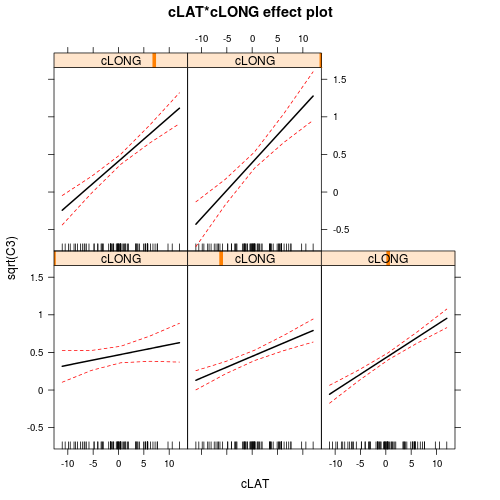
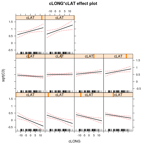
There is clearly an interaction between LAT and LONG. This indicates that the degree to which latitude effects the relative abundance of C3 plants depends on longitude and vice versa. The effects plots expressed for Latitude suggest that the relationship between relative C3 abundance and Latitude increases with increasing Longitude. The effects plots expressed for Longitude suggest that the relationship between relative C3 abundance and Longitude switch from negative at low Latitudes to positive at high Latitudes.
- Calculate the five levels of longitude on which the simple effects of latitude will be investigated. (HINT, HINT, etc).
Show code
> LongM2 <- mean(paruelo$cLONG) - 2 * sd(paruelo$cLONG) > LongM1 <- mean(paruelo$cLONG) - 1 * sd(paruelo$cLONG) > LongM <- mean(paruelo$cLONG) > LongP1 <- mean(paruelo$cLONG) + 1 * sd(paruelo$cLONG) > LongP2 <- mean(paruelo$cLONG) + 2 * sd(paruelo$cLONG) - Investigate the simple effects of latitude on the relative abundance of C3 plants for each of these levels of longitude. (HINT), (HINT), etc).
Show code
> LatM2 <- summary(paruelo.lmM2 <- lm(sqrt(C3) ~ cLAT * c(cLONG + > LongM2), data = paruelo))$coef["cLAT", ] > LatM1 <- summary(paruelo.lmM2 <- lm(sqrt(C3) ~ cLAT * c(cLONG + > LongM1), data = paruelo))$coef["cLAT", ] > LatM <- summary(paruelo.lmM2 <- lm(sqrt(C3) ~ cLAT * c(cLONG + > LongM), data = paruelo))$coef["cLAT", ] > LatP1 <- summary(paruelo.lmM2 <- lm(sqrt(C3) ~ cLAT * c(cLONG + > LongP1), data = paruelo))$coef["cLAT", ] > LatP2 <- summary(paruelo.lmM2 <- lm(sqrt(C3) ~ cLAT * c(cLONG + > LongP2), data = paruelo))$coef["cLAT", ] > rbind(`Lattitude at Long-2sd` = LatM2, `Lattitude at Long-1sd` = LatM1, > `Lattitude at mean Long` = LatM, `Lattitude at Long+1sd` = LatP1, > `Lattitude at Long+2sd` = LatP2) Estimate Std. Error t value Pr(>|t|)Lattitude at Long-2sd 0.07307061 0.012418103 5.884200 1.301574e-07Lattitude at Long-1sd 0.05838215 0.008113745 7.195463 5.877401e-10Lattitude at mean Long 0.04369369 0.004867032 8.977481 3.279384e-13Lattitude at Long+1sd 0.02900523 0.005270175 5.503657 5.926168e-07Lattitude at Long+2sd 0.01431678 0.008837028 1.620090 1.097748e-01
Multiple Linear Regression
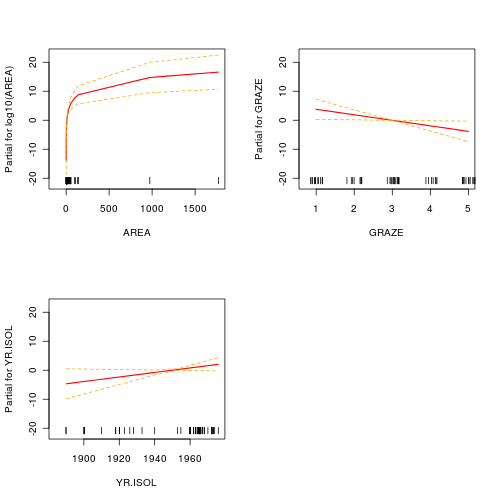
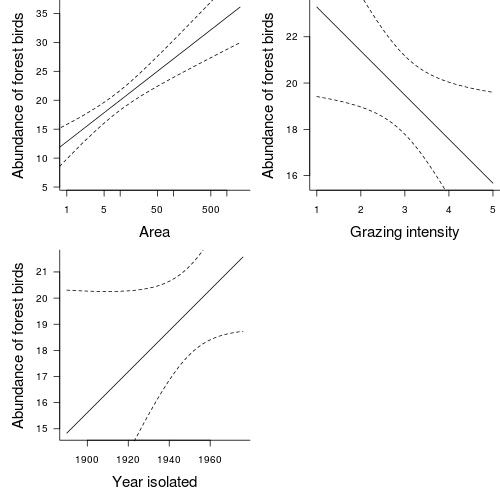
Loyn (1987) modeled the abundance of forest birds with six predictor variables (patch area, distance to nearest patch, distance to nearest larger patch, grazing intensity, altitude and years since the patch had been isolated).
Download Loyn data set
| Format of loyn.csv data file | |||||||||||||||||||||||||||||
|---|---|---|---|---|---|---|---|---|---|---|---|---|---|---|---|---|---|---|---|---|---|---|---|---|---|---|---|---|---|
|
 |
| Assumption | Diagnostic/Risk Minimization |
|---|---|
| I. | |
| II. | |
| III. | |
| IV. | |
| V. |
- Focussing on the assumptions of Normality, Homogeneity of Variance and Linearity, is there evidence of violations of these assumptions (y or n)?
- Try applying a temporary log10 transformation to the skewed variables(HINT).
Show codeDoes this improve some of these specific assumptions (y or n)?
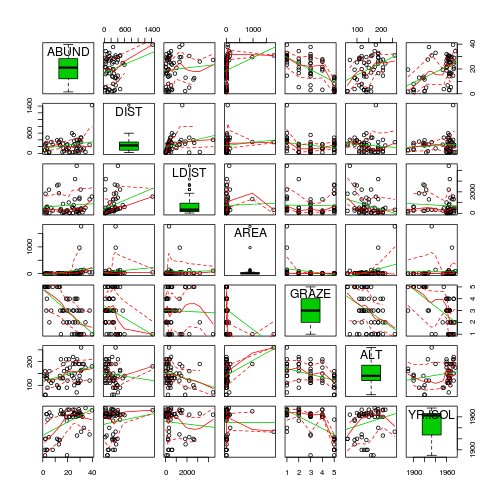
> library(car) > scatterplotMatrix(~ABUND + log10(DIST) + log10(LDIST) + log10(AREA) + > GRAZE + ALT + YR.ISOL, data = loyn, diagonal = "boxplot") 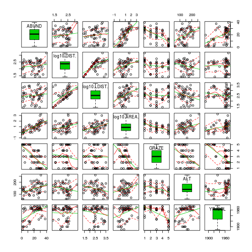
- Is there any evidence that the assumption of Collinearity is likely to be violated (y or n)?
Show code
> loyn.lm <- lm(ABUND ~ log10(DIST) + log10(LDIST) + log10(AREA) + > GRAZE + ALT + YR.ISOL, data = loyn) > vif(loyn.lm) log10(DIST) log10(LDIST) log10(AREA) GRAZE ALT YR.ISOL1.654553 2.009749 1.911514 2.524814 1.467937 1.804769> 1/vif(loyn.lm) log10(DIST) log10(LDIST) log10(AREA) GRAZE ALT YR.ISOL0.6043930 0.4975746 0.5231454 0.3960688 0.6812282 0.5540876
Predictor VIF Tolerance log10(DIST) log10(LDIST) log10(AREA) GRAZE ALT YR.ISOL - Collinearity typically occurs when one or more of the predictor variables are correlated, therefore this assumption can also be examined by calculating the pairwise correlation coefficients between all the predictor variables (use transformed versions for those that required it) (
HINT).
Show codeNone of the predictor variables are overly correlated to any of the other predictor variables.
> cor(loyn.lm$model[, 2:7]) log10(DIST) log10(LDIST) log10(AREA) GRAZE ALTlog10(DIST) 1.00000000 0.60386637 0.3021666 -0.14263922 -0.2190070log10(LDIST) 0.60386637 1.00000000 0.3824795 -0.03399082 -0.2740438log10(AREA) 0.30216662 0.38247952 1.0000000 -0.55908864 0.2751428GRAZE -0.14263922 -0.03399082 -0.5590886 1.00000000 -0.4071671ALT -0.21900701 -0.27404380 0.2751428 -0.40716705 1.0000000YR.ISOL -0.01957223 -0.16111611 0.2784145 -0.63556710 0.2327154YR.ISOLlog10(DIST) -0.01957223log10(LDIST) -0.16111611log10(AREA) 0.27841452GRAZE -0.63556710ALT 0.23271541YR.ISOL 1.00000000
Since none of the predictor variables are highly correlated to one another, we can include all in the linear model fitting.
In this question, we are not so interested in hypothesis testing. That is, we are not trying to determine if there is a significant effect of one or more predictor variables on the abundance of forest birds. Rather, we wish to either (or both);
- Construct a predictive model for relating habitat variables to forest bird abundances
- Determine which are the most important (influential) predictor variables of forest bird abundances
- Examine the diagnostic plots (HINT) specially the residual plot to confirm no further evidence of violations of the analysis assumptions
Show code
> par(mfrow = c(2, 3), oma = c(0, 0, 2, 0)) > plot(loyn.lm, ask = F, which = 1:6) 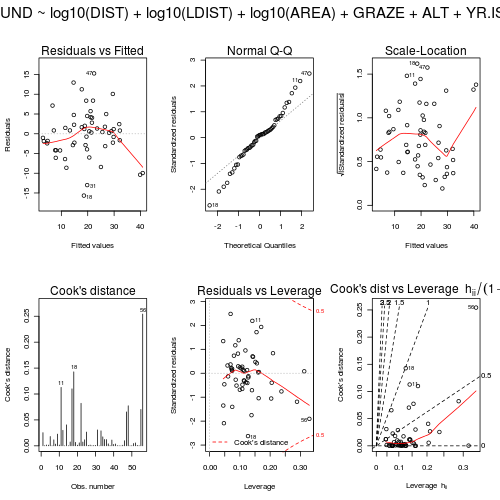
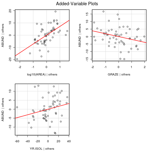
> influence.measures(loyn.lm) Influence measures oflm(formula = ABUND ~ log10(DIST) + log10(LDIST) + log10(AREA) + GRAZE + ALT + YR.ISOL, data = loyn) :dfb.1_ dfb.l10.D dfb.l10.L dfb.l10.A dfb.GRAZ dfb.ALT dfb.YR.I1 -0.024547 0.08371 -0.022664 0.325348 0.219000 -0.005547 0.0084682 -0.017509 -0.01656 0.020997 0.012653 0.003658 0.037247 0.0160133 -0.058912 0.01045 -0.016321 0.048309 0.012241 -0.021952 0.0609044 -0.024649 -0.01083 -0.015504 -0.047360 -0.005965 0.010247 0.0283275 0.064514 0.17236 -0.075678 -0.091673 0.105181 0.101385 -0.0784066 -0.013955 0.01154 0.003907 -0.027075 -0.003667 0.000920 0.0141847 0.152729 -0.14223 0.018225 0.056318 -0.149535 0.022629 -0.1484868 -0.012535 0.00936 -0.059652 0.050580 -0.001515 0.058081 0.0124669 0.240434 -0.10307 0.040989 0.142365 -0.165009 -0.019501 -0.24385410 -0.049652 -0.03654 -0.001350 0.035981 -0.001217 -0.021708 0.05413111 0.326311 -0.29680 0.393485 -0.464543 -0.259851 0.555537 -0.34714912 -0.318813 -0.04143 0.184910 -0.047393 0.001434 -0.058520 0.32466913 -0.003880 -0.00858 -0.003634 -0.013295 -0.006816 0.013654 0.00485314 0.049590 -0.19049 -0.118128 0.391650 0.193189 -0.285935 -0.03384115 0.028372 0.01892 -0.019252 0.001533 0.002733 -0.003094 -0.02940616 -0.112157 0.03131 -0.058961 0.040297 -0.017552 -0.062221 0.11965717 0.089920 -0.36895 -0.418556 0.197950 -0.137942 -0.554335 -0.01692918 0.003210 0.44969 0.471153 -0.189555 0.055517 0.413749 -0.08160419 -0.014516 -0.05622 -0.077388 0.014877 0.026729 0.051520 0.02149320 0.031138 0.01561 -0.029390 -0.019603 -0.059824 -0.066354 -0.02644521 -0.074573 0.03497 0.084655 -0.115333 0.004721 0.153777 0.06622922 0.012462 0.62313 -0.547520 0.034210 -0.102778 0.004117 -0.02062123 0.007417 0.07767 0.112948 -0.066606 0.000558 0.110277 -0.02412324 0.057330 0.06179 -0.042947 -0.103211 -0.203842 -0.153868 -0.04605525 0.399742 -0.06158 -0.055316 -0.020120 -0.228704 0.012557 -0.40010726 -0.036316 -0.02478 0.062377 -0.032586 0.009891 0.023836 0.03530227 0.062196 -0.01369 -0.045659 0.029139 -0.023443 -0.004247 -0.06113628 0.022345 -0.01170 0.005156 -0.004665 -0.032184 -0.032509 -0.02056529 -0.048454 0.02411 -0.016234 0.017630 0.047216 -0.006470 0.04855030 0.020424 0.00550 0.013709 0.018552 0.021831 -0.019583 -0.02232231 0.181882 -0.18332 0.070644 -0.044548 -0.080909 0.204938 -0.18899332 -0.004554 -0.00646 -0.010581 0.012558 0.011367 0.000130 0.00533933 -0.192246 0.07100 -0.214312 0.246055 0.262466 -0.178104 0.20526534 -0.167748 0.08351 -0.072012 0.100394 0.263665 0.204739 0.15663235 0.056797 -0.06516 0.082675 0.005839 0.006404 -0.128022 -0.05677336 -0.136228 -0.06411 0.004602 0.101551 0.082178 -0.132967 0.14867837 0.004153 -0.01116 -0.045478 -0.053435 -0.081659 0.014926 0.00137238 -0.010846 -0.04066 0.048479 -0.013496 -0.004557 0.016275 0.01088339 -0.222802 0.01356 0.109160 0.039879 0.210745 0.089951 0.21431740 -0.005977 0.01113 -0.036499 -0.056239 -0.058831 0.032006 0.00864341 -0.031032 -0.08019 0.031978 0.020113 0.089394 0.033669 0.03056642 -0.029798 0.03356 -0.007763 0.018255 0.027276 -0.002476 0.02846543 0.001060 -0.00833 0.008234 -0.000729 0.011017 -0.007667 -0.00124944 0.004393 -0.00930 0.000714 0.002619 -0.009448 -0.010691 -0.00325445 0.011664 0.03240 -0.064340 0.046954 -0.013554 -0.053380 -0.00815646 -0.044055 0.00853 -0.126785 0.175238 0.125507 0.057840 0.04517847 0.348086 -0.09628 0.068676 0.328440 -0.113019 -0.256880 -0.34765548 -0.139098 0.50451 0.055716 -0.138456 -0.085820 0.270712 0.10390449 0.000830 0.00124 0.009247 -0.002171 -0.015170 -0.005737 -0.00063550 0.010389 0.02638 -0.015605 0.006676 -0.022689 -0.000897 -0.01072651 -0.048345 -0.13467 0.071349 0.066280 0.022910 0.002208 0.05372952 -0.019314 0.04851 -0.061717 -0.025118 0.088505 0.129007 0.01252053 -0.000455 -0.00517 -0.030151 -0.009949 0.025032 -0.004643 0.00186054 0.032378 -0.00621 -0.010783 0.019668 -0.025119 -0.000179 -0.03192755 0.072633 -0.00990 -0.045849 -0.458184 -0.072288 -0.111714 -0.06076756 -0.524582 -0.31857 0.429361 -0.754208 0.024705 -0.528460 0.569683dffit cov.r cook.d hat inf1 -0.4206 1.395 2.55e-02 0.23742 -0.0657 1.319 6.29e-04 0.12793 -0.1103 1.288 1.77e-03 0.11504 0.0998 1.217 1.45e-03 0.06905 0.3575 1.036 1.81e-02 0.08496 0.0385 1.243 2.16e-04 0.07347 -0.2837 1.250 1.16e-02 0.13998 -0.1520 1.289 3.36e-03 0.12479 -0.4029 0.937 2.27e-02 0.074810 -0.1064 1.286 1.65e-03 0.113211 0.9263 0.653 1.13e-01 0.141312 -0.4586 1.179 3.00e-02 0.162013 0.0364 1.302 1.93e-04 0.114214 -0.5334 1.236 4.06e-02 0.203615 0.0490 1.295 3.50e-04 0.110516 -0.2278 1.199 7.50e-03 0.099817 0.9038 0.798 1.10e-01 0.170418 -1.0674 0.459 1.43e-01 0.1268 *19 0.2163 1.162 6.75e-03 0.080420 0.0950 1.281 1.31e-03 0.107821 0.1998 1.318 5.80e-03 0.151322 -0.7615 1.323 8.21e-02 0.288823 -0.2259 1.218 7.38e-03 0.107924 0.2864 1.253 1.18e-02 0.141925 0.4310 1.320 2.67e-02 0.209526 0.0810 1.209 9.54e-04 0.059127 -0.1034 1.178 1.55e-03 0.048728 -0.0462 1.322 3.11e-04 0.128129 0.0678 1.284 6.70e-04 0.105330 0.0809 1.272 9.54e-04 0.099831 -0.4816 0.632 3.08e-02 0.047232 0.0235 1.380 8.04e-05 0.163033 0.4545 0.968 2.89e-02 0.096234 0.3493 1.149 1.75e-02 0.118335 -0.2959 0.929 1.23e-02 0.045236 0.2943 0.930 1.22e-02 0.044937 -0.1651 1.254 3.96e-03 0.108538 0.0559 1.679 4.56e-04 0.3127 *39 0.2799 1.260 1.13e-02 0.143540 -0.1378 1.287 2.76e-03 0.120441 -0.1590 1.221 3.67e-03 0.088842 0.0597 1.236 5.19e-04 0.071443 -0.0327 1.228 1.56e-04 0.061144 0.0161 1.376 3.79e-05 0.160445 0.0934 1.260 1.27e-03 0.094346 0.2630 1.157 9.95e-03 0.093647 0.7168 0.485 6.55e-02 0.0693 *48 0.7515 0.885 7.74e-02 0.155049 0.0297 1.246 1.28e-04 0.074650 0.0536 1.242 4.18e-04 0.074451 0.1778 1.335 4.60e-03 0.156152 -0.1989 1.421 5.75e-03 0.205253 -0.0817 1.251 9.72e-04 0.086254 0.0506 1.315 3.73e-04 0.124055 -0.7173 0.853 7.03e-02 0.138456 -1.3723 1.007 2.54e-01 0.3297 * - On initial examination of the fitted model summary, which of the predictor variables might
you consider important? (this can initially be determined by exploring which of the effects are significant?)
Show code> summary(loyn.lm) Call:lm(formula = ABUND ~ log10(DIST) + log10(LDIST) + log10(AREA) +GRAZE + ALT + YR.ISOL, data = loyn)Residuals:Min 1Q Median 3Q Max-15.6506 -2.9390 0.5289 2.5353 15.2842Coefficients:Estimate Std. Error t value Pr(>|t|)(Intercept) -125.69725 91.69228 -1.371 0.1767log10(DIST) -0.90696 2.67572 -0.339 0.7361log10(LDIST) -0.64842 2.12270 -0.305 0.7613log10(AREA) 7.47023 1.46489 5.099 5.49e-06 ***GRAZE -1.66774 0.92993 -1.793 0.0791 .ALT 0.01951 0.02396 0.814 0.4195YR.ISOL 0.07387 0.04520 1.634 0.1086---Signif. codes: 0 ‘***’ 0.001 ‘**’ 0.01 ‘*’ 0.05 ‘.’ 0.1 ‘ ’ 1Residual standard error: 6.384 on 49 degrees of freedomMultiple R-squared: 0.6849, Adjusted R-squared: 0.6464F-statistic: 17.75 on 6 and 49 DF, p-value: 8.443e-11
Coefficient Estimate t-value P-value Intercept log10(DIST) log10(LDIST) log10(AREA) GRAZE ALT YR.ISOL
Clearly, not all of the predictor variables have significant partial effects on the abundance of forest birds. In developing a predictive model for relating forest bird abundances to a range of habitat characteristics, not all of the measured variables are useful. Likewise, the measured variables are not likely to be equally influential in determining the abundance of forest birds.
| Model | Adj. r2 | AIC | BIC |
|---|---|---|---|
| Full |
- The model that you would consider to be the most parsimonious would be the model containing which terms?
- Use the model averaging to estimate the regression coefficients for each term.
Predictor: Estimate SE Lower 95% CI Upper 95% CI log10 patch distance log10 large patch distance log10 fragment area Grazing intensity Altitude Years of isolation Intercept
- the model averaging
- refitting the most parsimonious model
Show code
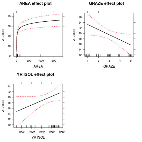
> loyn.lm1 <- lm(ABUND ~ log10(AREA) + GRAZE + YR.ISOL, data = loyn) > summary(loyn.lm1) Call:lm(formula = ABUND ~ log10(AREA) + GRAZE + YR.ISOL, data = loyn)Residuals:Min 1Q Median 3Q Max-14.5159 -3.8136 0.2027 3.1271 14.5542Coefficients:Estimate Std. Error t value Pr(>|t|)(Intercept) -134.26065 86.39085 -1.554 0.1262log10(AREA) 7.16617 1.27260 5.631 7.32e-07 ***GRAZE -1.90216 0.87447 -2.175 0.0342 *YR.ISOL 0.07835 0.04340 1.805 0.0768 .---Signif. codes: 0 ‘***’ 0.001 ‘**’ 0.01 ‘*’ 0.05 ‘.’ 0.1 ‘ ’ 1Residual standard error: 6.311 on 52 degrees of freedomMultiple R-squared: 0.6732, Adjusted R-squared: 0.6544F-statistic: 35.71 on 3 and 52 DF, p-value: 1.135e-12
Polynomial regression
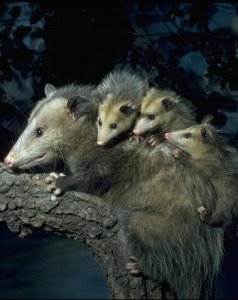
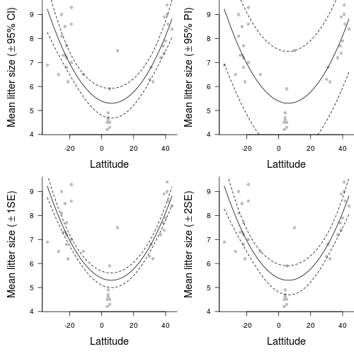
Rademaker and Cerqueira (2006), compiled data from the literature on the reproductive traits of opossoms (Didelphis) so as to investigate latitudinal trends in reproductive output. In particular, they were interested in whether there were any patterns in mean litter size across a longitudinal gradient from 44oN to 34oS. Analyses of data compiled from second hand sources are called metaanalyses and are very usefull at revealing overal trends across a range of studies.
Download Rademaker data set
| Format of rademaker.csv data files | |||||||||||||||||||||||||||||||||||||||||||||||||||||||
|---|---|---|---|---|---|---|---|---|---|---|---|---|---|---|---|---|---|---|---|---|---|---|---|---|---|---|---|---|---|---|---|---|---|---|---|---|---|---|---|---|---|---|---|---|---|---|---|---|---|---|---|---|---|---|---|
|
 |
||||||||||||||||||||||||||||||||||||||||||||||||||||||
The main variables of interest in this data set are MLS (mean litter size) and LATITUDE. The other variables were included so as to enable you to see how meta data might be collected and collated from a number of other sources.
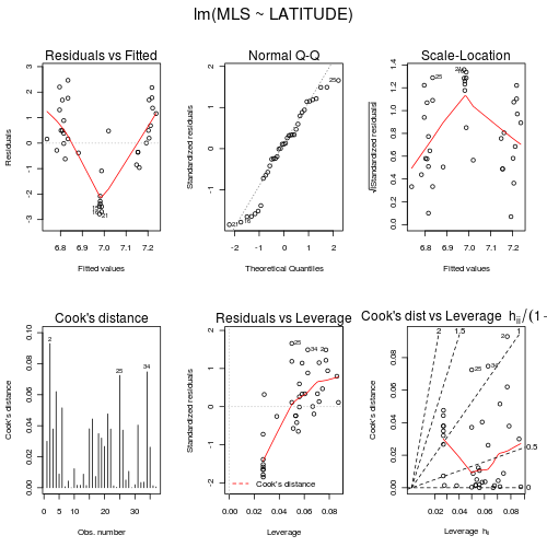
The relationship between two continuous variables can be analyzed by simple linear regression. Before performing the analysis we need to check the assumptions. To evaluate the assumptions of linearity, normality and homogeneity of variance, construct a scatterplot of MLS against LATITUDE including a lowess smoother and boxplots on the axes. (HINT)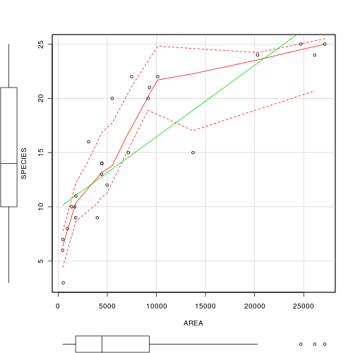
| DV | = | intercept | + | slope1 | x | IV2 | + | slope2 | x | IV |
|---|---|---|---|---|---|---|---|---|---|---|
| Mean litter size | = | + | x | latitude2 | + | x | latitude |
- The slopes
significantly different from one another and to 0 (F =
, df =
,
, P =
)
- The second order polynomial regression model
fit the data significantly better than a first order (straight line) regression model (F =
, FONT face=Courier>df =
,
, P =
)
Nonlinear Regression
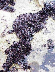
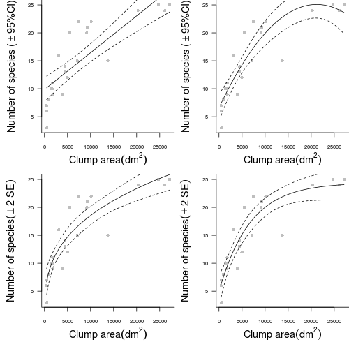
Peake and Quinn (1993) investigated the relationship between the size of mussel clumps (m2) and the number of other invertebrate species supported.
Download Peake data set
| Format of peake.csv data file | ||||||||||||||||||||||
|---|---|---|---|---|---|---|---|---|---|---|---|---|---|---|---|---|---|---|---|---|---|---|
|
 |
- Focussing on the assumptions of Normality, Homogeneity of Variance and Linearity, is there evidence of violations of these assumptions (y or n)?
- Try fitting a second order
polynomial trendline
through these data. E.g. Species = α*Area + β*Area2 + c (note that this is just an extension of y=mx+c)
Show code
> peake.lm <- lm(SPECIES ~ AREA + I(AREA^2), data = peake) - Try fitting a power trendline
through these data. E.g. Species = α(Area)β where the number of Species is proportional to the Area to the power of some coefficient (β).
Show code
> peake.nls <- nls(SPECIES ~ alpha * AREA^beta, data = peake, start = list(alpha = 0.1, > beta = 1)) - Try fitting an asymptotic exponential relationship through these data. E.g. Species = α-βeγArea.
Show code
> peake.nls1 <- nls(SPECIES ~ SSasymp(AREA, a, b, c), data = peake)
| Model | AIC | MSresid | P-value |
|---|---|---|---|
| Species = β*Area + c | Compare linear and polynomial in the box below |
||
| Species = α*Area + β*Area2 + c | |||
| Species = α(Area)β | Compare power and asymptotic exponential in the box below |
||
| Species = α-βeγArea |
- Start by setting up some whole figure (graphics device) parameters. In particular, indicate that the overall figure is going to comprise 2 rows and 2 columns.
Show code
> opar <- par(mfrow = c(2, 2)) - Setup the margins (5 units on the bottom and left and 0 units on the top and right) and dimensions of the blank plotting space. Also add the raw observations as solid grey dots
Show code
> opar1 <- par(mar = c(5, 5, 0, 0)) > plot(SPECIES ~ AREA, data = peake, ann = F, axes = F, type = "n") > points(SPECIES ~ AREA, data = peake, col = "grey", pch = 16) - Use the predict function to generate predicted (fitted) values and 95% confidence intervals for 1000 new AREA values between the minimum and maximum original AREA range. Plot the trend and confidence intervals in solid and dotted lines respectively.
Show code
> xs <- with(peake, seq(min(AREA), max(AREA), l = 1000)) > ys <- predict(peake.lmLin, data.frame(AREA = xs), interval = "confidence") > points(ys[, "fit"] ~ xs, col = "black", type = "l") > points(ys[, "lwr"] ~ xs, col = "black", type = "l", lty = 2) > points(ys[, "upr"] ~ xs, col = "black", type = "l", lty = 2) - Add axes, axes titles and a "L" shape axes box to the plot to complete the first sub-figure
Show code
> axis(1, cex.axis = 0.75) > mtext(expression(paste("Clump area", (dm^2))), 1, line = 3, cex = 1.2) > axis(2, las = 1, cex.axis = 0.75) > mtext(expression(paste("Number of species (", phantom() %+-% > 95, "%CI)")), 2, line = 3, cex = 1.2) > box(bty = "l") > par(opar1) - Complete the second sub-figure (polynomial trend) in much the same manner as the first (linear trend)
Show code
> opar1 <- par(mar = c(5, 5, 0, 0)) > plot(SPECIES ~ AREA, data = peake, ann = F, axes = F, type = "n") > points(SPECIES ~ AREA, data = peake, col = "grey", pch = 16) > xs <- with(peake, seq(min(AREA), max(AREA), l = 1000)) > ys <- predict(peake.lm, data.frame(AREA = xs), interval = "confidence") > points(ys[, "fit"] ~ xs, col = "black", type = "l") > points(ys[, "lwr"] ~ xs, col = "black", type = "l", lty = 2) > points(ys[, "upr"] ~ xs, col = "black", type = "l", lty = 2) > axis(1, cex.axis = 0.75) > mtext(expression(paste("Clump area", (dm^2))), 1, line = 3, cex = 1.2) > axis(2, las = 1, cex.axis = 0.75) > mtext(expression(paste("Number of species (", phantom() %+-% > 95, "%CI)")), 2, line = 3, cex = 1.2) > box(bty = "l") > par(opar1) - Start the third (power) model similarly
Show code
> opar1 <- par(mar = c(5, 5, 0, 0)) > plot(SPECIES ~ AREA, data = peake, ann = F, axes = F, type = "n") > points(SPECIES ~ AREA, data = peake, col = "grey", pch = 16) - Estimating confidence intervals is a little more complex for non-linear least squares models as the predict() function does not yet support calculating standard errors or intervals.
Nevertheless, we can do this manually (go R you good thing!).
- Firstly we need to refit the non-linear power model incorporating a function that will be used to specify gradient calculations. This will be necessary to form the basis of SE calculations. So the gradient needs to be specified using the deriv3() function.
- Secondly, we then refit the power model using this new gradient function
Show code> grad <- deriv3(~alpha * AREA^beta, c("alpha", "beta"), function(alpha, > beta, AREA) NULL) > peake.nls <- nls(SPECIES ~ grad(alpha, beta, AREA), data = peake, > start = list(alpha = 0.1, beta = 1)) - The predicted values of the trend as well as standard errors can then be calculated and used to plot approximate 95% confidence intervals. One standard error is equivalent to approximately 68% confidence intervals. The conversion between standard error and 95% confidence interval follows the formula 95%CI=1.96xSE. Actually, 1.96 (or 2) is an approximation from large (>30) sample sizes. A more exact solution can be obtained by multiplying the SE by
pt(0.975,df)where df is the degrees of freedom.Show code> ys <- predict(peake.nls, data.frame(AREA = xs)) > se.fit <- sqrt(apply(attr(predict(peake.nls1, list(AREA = xs)), > "gradient"), 1, function(x) sum(vcov(peake.nls1) * outer(x, > x)))) > points(ys ~ xs, col = "black", type = "l") > points(ys + 2 * se.fit ~ xs, col = "black", type = "l", lty = 2) > points(ys - 2 * se.fit ~ xs, col = "black", type = "l", lty = 2) - Finish sub-figure 3 similar to the other two
Show code
> points(ys + 2 * se.fit ~ xs, col = "black", type = "l", lty = 2) > points(ys - 2 * se.fit ~ xs, col = "black", type = "l", lty = 2) > axis(1, cex.axis = 0.75) > mtext(expression(paste("Clump area", (dm^2))), 1, line = 3, cex = 1.2) > axis(2, las = 1, cex.axis = 0.75) > mtext(expression(paste("Number of species", (phantom() %+-% 2 ~ > SE), )), 2, line = 3, cex = 1.2) > box(bty = "l") > par(opar1) - Sub-figure four (asymptotic exponential) is similar to the power model except that as it already incorporates a gradient function (
SSasymp()), this step is not required.Show code> opar1 <- par(mar = c(5, 5, 0, 0)) > plot(SPECIES ~ AREA, data = peake, ann = F, axes = F, type = "n") > points(SPECIES ~ AREA, data = peake, col = "grey", pch = 16) > xs <- with(peake, seq(min(AREA), max(AREA), l = 1000)) > ys <- predict(peake.nls1, data.frame(AREA = xs)) > se.fit <- sqrt(apply(attr(ys, "gradient"), 1, function(x) sum(vcov(peake.nls1) * > outer(x, x)))) > points(ys ~ xs, col = "black", type = "l") > points(ys + 2 * se.fit ~ xs, col = "black", type = "l", lty = 2) > points(ys - 2 * se.fit ~ xs, col = "black", type = "l", lty = 2) > axis(1, cex.axis = 0.75) > mtext(expression(paste("Clump area", (dm^2))), 1, line = 3, cex = 1.2) > axis(2, las = 1, cex.axis = 0.75) > mtext(expression(paste("Number of species", (phantom() %+-% 2 ~ > SE), )), 2, line = 3, cex = 1.2) > box(bty = "l") > par(opar1) - Finally, finalize the figure by restoring the plotting (graphics device) parameters
Show code
> par(opar)
TODO - put in GAM and regression tree examples