This section illustrates the role of an impermeable layer (a seal) in focusing regional scale fluid flow, and its implications to mineralizaton. The models reveal how a simple horizontal permeability change alone between layers can cause crustal scale disturbance during a deformation event accompanied by fluid influx into the system. Fluid will migrate upwards preferentially along the contact between the two layers of contrasting permeability, as a result of the high pore pressure developed under the sealing layer. This high pore pressure also leads to yielding in tension and the jacking up of the sealing layer, as well as yielding in shear. When differences in the elastic or plastic rock properties are added to the system straining of the vertical or steep contact between the two layers, leads to yielding and further focusing of the upward fluid flow transport to the contact zone. When permeability function is added to the system that increases permeability of the material upon yielding (Figs 4 and 5), fluid flow at the contact zone is further intensified.
The model is a vertical crustal section, 30 km wide and 10 km deep with fluid saturating pores and initially at hydrostatic pore pressure. The entire model consists of a homogeneously permeable rock except for a layer in the upper half of the model which consists of a low permeability layer, an effective barrier for fluid flow. The models explore regional fluid flow during horizontal shortening as a constant fluid discharge is imposed at the base, analogue to fluids released through regional metamorphism. These models were designed to explore the role of impermeable layers for mineralizing systems. The permeability of each area is thought to represent, not a laboratory measure of rock permeability, but as simulating an averaged value of the regional permeability of the rock succession, including structural permeability such as that provided by shear zones, fractures, irregular rock contacts.
Figure 1. A) Model set up. The low-permeability layer on the right-hand-side may have either a steeply dipping contact with the high-permeability contact (as shown), or a vertical contact. The permeabilities for both layers were chosen to be very low, which results in slow fluid flow velocities. The high-permeability layer is 104 times more permeable than the low-permeability layer. B) Model set up for Figure 8, with low-permeability irregular bodies, randomly places in the left-hand-side of the model and embedded in a high-permeability background. This model has similar dimensions and fluid discharge at the base.
A) Seal Model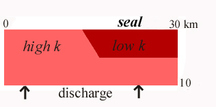 |
B) Low Permeability
Bodies
|
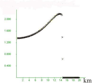
Figure 2. Model 2 has a vertical contact between the two layers and they have the same physical properties except for permeabilities, so that yielding is related to differential pore pressures and consequent differences in effective stress resulting from the permeability contrast. In this model, permeability is constant whether or not the material is at yield, and the model surface is at a pressure of 2 kb. A) Hydraulic uplifting (see embedded movie) of the low-permeability layer on the right-hand-side, accompanied by intense yielding of the material underlying it. B) Pore pressure evolution (see embedded movie). Note pore pressure increase under the low permeability layer which accompanies its uplifting and fracturing. High pore pressure leads to low effective stress and yielding under shear (red in A) or tension (yellow in A). Note also that the pore pressure contours are not horizontal as it would be in equilibrium but they slope, causing lateral fluid flow (at right angles to contour lines) from underneath the low-permeability layer towards the left. C) Lateral fluid escape from the high pore pressure region underneath the low-permeability layer leads to fastest fluid flow (in deep green, blue and white in the figure) close to the boundary between the two layers. D) Horizontal velocity profile, from left to right, close to the top surface of the model, showing a two-fold increase in fluid velocity towards the contact of the two layers, followed by a sharp decrease in the low-permeability layer on the right-hand-side.
A) State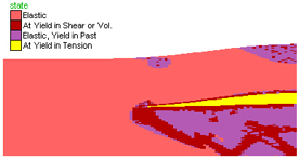 |
B) Pore pressure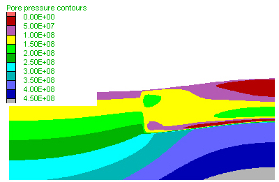 |
C) Flow velocity 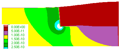 |
D)
Flow velocity at surface 10-10m/s
 |
Input file
Figure 3. Model 5 has a sloping contact between the two layers. The low-permeability layer has bulk modulus one order of magnitute higher than the high-permeability layer, and lower cohesion and tension. These differences translate into an elastically stronger but plastically weaker low-permeability layer, tending to yield at lower differential stresses than the high permeability. Like Model 2 there is no permeability change upon yielding. The results are essentially similar to those of Model 2, except for yielding of the plastically weaker low-permeability layer, including yielding along the sloping contact. Note in D) that flow velocity increases three-fold within the high-permeability layer, towards the contact. Note also that the flow velocity in the high-permeability layer, away from the contact approaches that estimated by Darcy's Law for the average pore pressure gradient across the model. This can be found by determining the pore pressure close to the base and close to the top of the model, and determining the average pore pressure gradient by dividing that difference by the total 10000 m depth of the layer. In this case pore pressure gradient equals (2.443e8 - 3.823e7)/10000m=2.443 e4 Pa/m, which yields a head gradient of 1.443 (by subtracting 1 corresponding to the pore pressure gradient at hydrostatic pressure). This yield a Darcy velocity equal to 1.4 e-10 (click here for more details).
A) State |
B) Pore pressure |
C) Flow velocity  |
D) Flow velocity at
surface 10-10m/s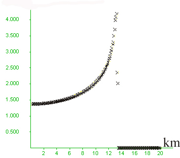
|
Input file
Figure 4. In the models presented so far, no permeability changes during the calculations were allowed. In Model 17 (200*100 resolution and identical to a lower, 100*100, resolution model 10, not shown here), which is essentially similar to Model 5, a FISH function was added that changes the permeability according to the state of the material. If the material is at yield in shear, permeability is increased by a factor of 20, if it has yielded any time in the past, but is not currently yielding the permeability is still higher than its initial permeability, but only by a factor of 10. If the material is at yield in tension, then permeability is increased by a factor of 50. In this model the same rule is applied for both layers, which means that the low-permeability layer will always have considerably lower permeability than the high-permeability layer. The pressure at the top of the model was decreased to 1 kb. Note also that in this model the total straining allowed was much smaller than that of previous models. A) Shortening of the sequence (click on figure for embedded movie) leads first to yielding of the low-permeability layer close to the contact, followed by the development of a new shear band, at a smaller angle. The shear band developed early in the low-permeability layer has negligible effect on the evolution of the system. The later shear band developed within high permeability rocks leads to considerable changes in the pore pressure distribution. B) Detail of pore pressure contours and high permeability zones (marked by the white lines) close to the contact. The high permeability shear band affects the pore pressure in its surroundings causing local deflections of the contour lines. As the shear band develops and rapidly tranports fluids upwards, it causes first a pressure drop at its base and pressure increase at its upwards propagating tip. Once the shear band reaches the top boundary of the model, than it leads to a generalized pressure decrease along its path, as can be seen on the static figure below, where the purple zone protrudes downwards into the yellow zone. The embedded movie zooms into a region close to the contact and shear bands.
A) State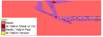 |
B) Pore pressure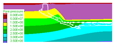 |
C)
Pore pressure detail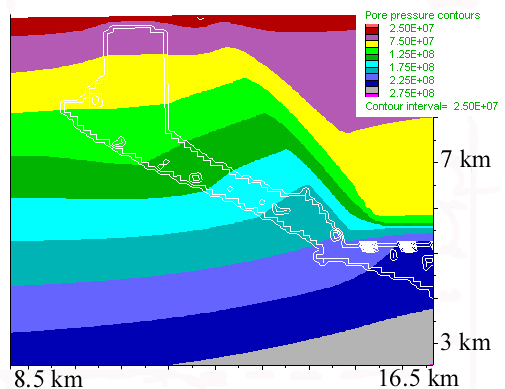 |
C) and D) Horizontal fluid flow velocity profiles close to the model surface. Notice the different y-axis scales. C) Before the development of the new, permeable shear zone. Like in Model 5, there is a moderate four-fold increase in flow velocity towards the contact, and fluid velocities are of the order of 10-10 m/s, but higher than in Model 5, due to yielding of the permeable layer close to the contact; D) Note change in scale of the y-axis. After the development of the new permeable shear band, the velocity peak increases significantly, while the flow velocity far away from the shear band remains constant. At this stage there is a lateral velocity increase by a factor of 6 in the permeable layer, left of and adjacent to the contact. Notice that the increase in fluid velocity is not proportional to the 10- or 20-fold increase in permeability. This is because fluid velocity (Darcy's Law) depends on permeability but also on the driving pore pressure gradient. The high permeability shear zone causes a decrease in the pore pressure gradient leading to a less sharp increase in fluid velocity.
C) Early flow velocity
profile 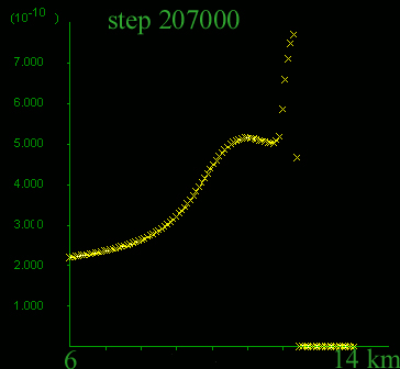
|
D)
Late flow velocity profile 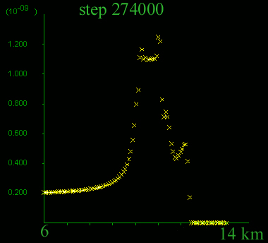
|
Input file
Figure 5. Model 15 is similar to Model 17 (Fig. 4) and tests the role of the contrast in permeability between the two layers. Here, k' is defined as the ratio between permeability of the two layers:
k'=kseal/kperm
In Fig. 4, k'=1.e4 (in other words the permeable layer is 10000 times more permeable than the seal). In model 15 this was reduced to 100, keeping all else equal. The results are considerably different. In this model, the decreased value of k' implies that the sealing layer is not as efficient. This leads to fluid flow through it, and this can be seen in the gradual increased in pore pressure within the sealing layer. This leakage of fluids into the sealing layer releases some of the pore pressure increase in the underlying layer so that less fluid is deflected to the left. The increase in pore pressure within the sealing layer causes it to yield further increasing permeability. As a consequence, the increase in pore presure in the high permeability layer close to the contact is much subdued inhibiting yielding.
A)
State. Step 140000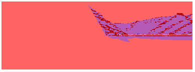 |
B)
Pore pressure. Step 140000 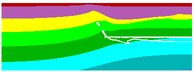
|
Input file
Figure 6. Model 11 is similar to Model 17 (Fig. 4) except that the FISH function that changes permeability according to material state has been modified. In Model 11, when both the high- and low-permeability layer yield in shear or in tension their permeability increase to 10-12, if it has yielded in the past the material permeability is more permeable than originally and is given a permeability of 10-13. For the high-permeability layer this represents a stronger increase in permeability than in Model 10, and for the low-permeability layer this is an extreme permeability increase. This model was designed to test the case where the elastically strong but plastically weak, low permeability layer yields and becomes the main fluid conductor. Because of its properties, the expectation is that the low-permeability layer on the right-hand-side will yield first and focus fluid flow.
A) Shortening of the sequence (click on figure for embedded movie) leads first to yielding of the low-permeability layer close to the contact. A shear band of high permeability develops close to the contact, totally within the originally low-permeability layer. Unlike Model 10 in Fig. 4, no new shear band develops within the high-permeability layer.
B) The high-permeability shear band within the low-perrmeability layer releases the high pore pressure developed underneath. This can be seen by following the boundary between the light and dark green colours in the movie. First that boundary rises as pore pressure increases, and then gradually recedes downwards and to the right as the high-permeability band develops and releases the high pore pressure. The white lines represent permeability contours, and mark approximately the original boundary between the two layers. Click on the figure to see embedded movie showing the pore pressure evolution within the region covered by the box in the figure.
A)
State |
B)
Pore pressure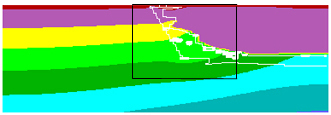 |
Click here for a full view movie
C) Fluid flow velocity (y-axis) section across the model close to its surface covering 7 km across the boundary between the two layers (x-axis). Note that the far-field fluid flow velocity remains close to the 2*10-10 as in Models 5 and 10, while the velocity within the high permeability shear zone is now 20 times that value. Notice also that the high-permeability fluid pathway is now over 2 km wide, and right of and adjacent to the contact. Comparison between the low and high resolution results (Figs 5 and 6) indicate that the results are qualitatively similar in their development, but quantitatively slightly different.
C) Step 160600 flow
velocity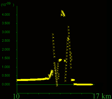
|
Input file
Figure 7. Model 12 is almost identical to Model 11 (Fig. 5) except that the grid resolution is higer at 300*200 (instead of 100*100) and the width of the box has been reduced from 30km to 28km.
A) Shortening of the sequence (click on figure for embedded movie) leads first to yielding of the low-permeability layer close to the contact. A shear band of high permeability develops close to the contact, totally within the originally low-permeability layer. Unlike Model 10 in Fig. 4, no new shear band develops within the high-permeability layer.
B) The high permeability shear band within the low-perrmeability layer releases the high pore pressure developed underneath the low-permeability layer. This can be seen by following the boundary between the light and dark green colours in the movie. First that boundary rises as pore pressure increases, and then gradually recedes downwards and to the right as the high-permeability band develops and releases the high pore pressure. The white lines represent permeability contours, and mark well the original boundary between the two layers. Click on the figure to see embedded movie showing the pore pressure evolution within the region covered by the box in the figure.
A) State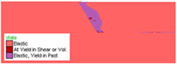 |
B) Pore pressure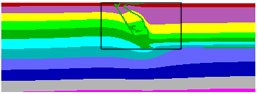 |
Click here for a full view movie
C) Fluid flow velocity distribution and D) horizontal section close to the model surface at different stages. The earliest stage on the left, velocity rises exponentially within the high-permeability material (on the left), towards the contact, even though no significant yielding has taken place. As yielding progresses, mostly within the low-permeability material to the right, permeability and fluid velocity increase as can be seen in C) by the widening of the zones in black. The widening of the high permeability zone also implies that considerable volumes of fluid are travelling through this high-permeability pathway. At the final step calculated (figure on the right-hand-side), fluid velocity increased five-fold close to the contact and is an order of magnitude higher than far field velocity. (The far-field fluid flow velocity remains close to the 2*10-10 as in Models 5, 10 and 11.) Note the different scales on the y-axis.
step 70600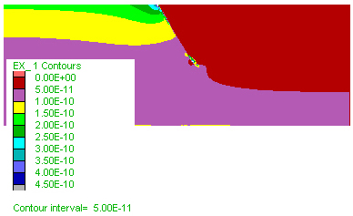 |
step 90600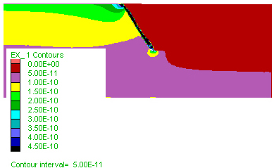 |
step 170600 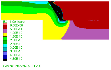
|
step 70600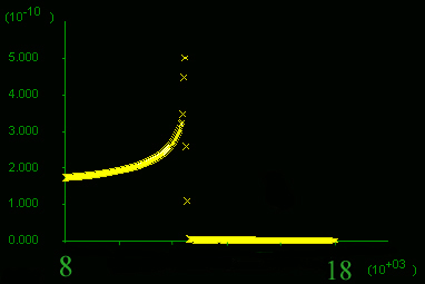
|
step 90600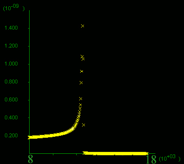
|
step 170600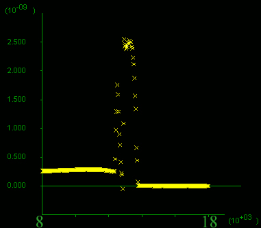
|
Input file
Figure 8. Early stages. Click on figures to see movies that show histories from begining to end and include figures 8, 9 and 10.
A) State. B) Pore pressure. High pore pressure on the left-hand-side of the model induced by the presence of the low-permeability bodies leads to early yielding and rapid fluid flow through fracture-related permeability increase. C) Integrated volume flux, showing highest flux at the margins of the low permeability bodies and in the left-hand-side of the model. D) Horizontal section across the top of the model showing variation in integrated volume flux, showing highest flux along fluid pathways in between the low-permeability bodies and at the boundary between the area with those bodies and the area to the right-handside free of those bodies. The distance between the flux peaks reflects the typical length scale of the low-permeability bodies.
A) step 32000 State
|
B) step 32000 Pore
pressure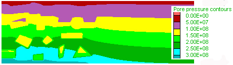
|
C) step 32000 Volume
flux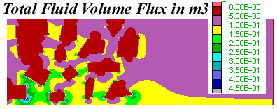
|
D) Volume flux section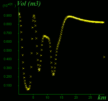
|
Figure 9. Intermediate stages. At this stage the left and the righ-hand-sides have yielded, though yielding is more developed in the left. High permeability in this area has lead to the release of pore pressure, leading to lower pore pressure on the left as compared to the right where late yielding has not released the pore pressure. C) and D) Shows the high flux on the left (yellow, green and blue colours). Note in D) how high volume flux peaks are accompanied by flux troughs and that the most intense peak is accompanied sideways by the lowest trough. High pore pressure on the right-hand-side leads to faster fluid velocity on the right.
step 64000 State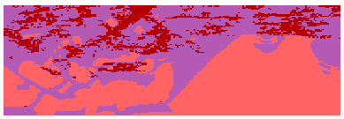
|
step 64000 Pore pressure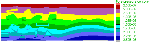
|
C) step 64000 Volume
flux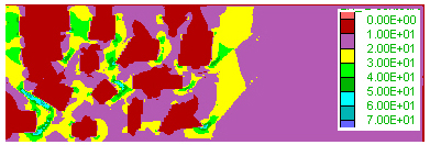
|
D) Volume flux section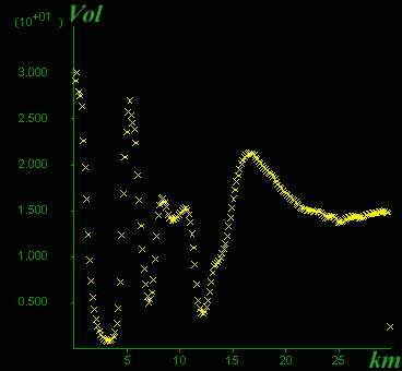
|
Figure 10. Late stages. Yielding-related permeability increase has released pore pressure, amd its lateral gradients. The vertical pore pressure gradient is approximately linear, except within the low-permeability bodies, and at this stage is lower than previously and 1.3 times hydrostatic pore pressure gradient.
step 124000 State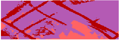
|
step 124000 Pore pressure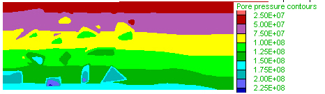
|
C) step 124000 Volume flux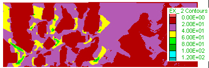
|
D) Volume flux section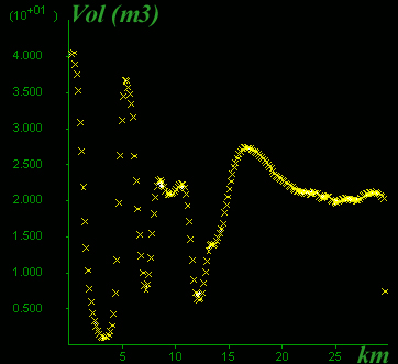
|
Input file
Figure 11. Vertical pore pressure (from top to base) at A) early (at 3km, left-hand-side), and B) late stages. During the early stages the pore pressure reaches nearly lithostatic pressure, whereas during the late stages the gradient is reduced to 1.3 times the hydrostatic pore pressure due to the high permeability channelways resulting from yielding. Note the different scales on the y-axis.
A) Step 32000 pore
pressure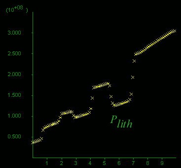 |
B) Step 124000 pore
pressure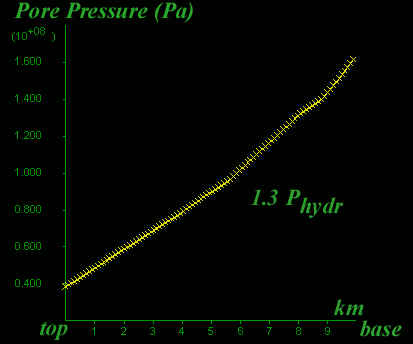 |
If yielding and associated increase in permeability is also considered the contact between the two packages will further focus fluid flow. Firstly, the contact zone between the two rock packages will yield before any other zone in the system because of the increased pore pressure compared to areas at similar depths.
Liked the structures? Want to know more? Contact me on my email