Preprint to: Comp. Appl. BioSci. (CABIOS), 9(1), pp.1-7, Feb 1993 (preprint.ps).
Partly
supported by Australian Research Council grant A49030439.
* To whom correspondence should be sent:
School of Computer Science, Monash University, Australia 3168.
A major use of string-alignment algorithms is to compare macro-molecules that are thought to have evolved from a common ancestor to estimate the duration of, or the amount of mutation in, their separate evolution and to infer as much as possible about their most recent common ancestor. Minimum Message Length encoding, a method of inductive inference, is applied to the string-alignment problem. It leads to an alignment method that averages over all alignments in a weighted fashion. Experiments indicate that this method can recover the actual parameters of evolution with high accuracy and over a wide range of values whereas the use of a single optimal alignment gives biased results.
Keywords: alignment, evolution, minimum message length encoding, MML, string similarity.
String-alignment algorithms are used to compare macro-molecules, that are thought to be related, to infer as much as possible about their most recent common ancestor and about the duration, amount and form of mutation in their separate evolution since diverging. A key question is how accurately and reliably can this be done. What can we reconstruct of the ancestor and the sequence of events that led to the given strings and how confident can we be in our inferences? Most string-alignment methods[Sank][Bish2] are based on finding an optimal alignment that minimises a cost function (or equivalently maximises a score) of some kind. Rare mutations are given a high cost. An alignment of two strings represents one possible evolutionary relationship, a set of possible ancestors and mutations, in a natural way. An optimal alignment represents, it might be hoped, a most probable relationship. However, we describe experiments that show that estimates of the parameters of the evolutionary process that are based on a single optimal alignment are biased, and that those derived from averaging over all alignments are not. Minimum Message Length (MML) techniques are used to estimate the parameters of the evolutionary process that gave rise to the strings.
MML encoding is a method of Bayesian inference. We consider the message length (ML) of an explanation of the given data. An explanation first states an hypothesis H, then states the data using a code which would be optimal if the hypothesis were true. From coding-theory, the message length in an optimal code of an event of probability P is -log2(P) bits. For an hypothesis H and data D, in the discrete case:
P(H&D) = P(H).P(D|H) = P(D).P(H|D) -- Bayes' theorem ML(H&D) = ML(H)+ML(D|H) = ML(D)+ML(H|D) |
P(H|D) is the posterior probability of hypothesis H given data D. The best hypothesis is the one that is part of the explanation having the shortest message length. We cannot in general talk about the true hypothesis, just "better" or "worse" hypotheses. The posterior odds-ratio of two hypotheses, H and H', can be calculated from the following:
ML(H|D)-ML(H'|D) = ML(H&D)-ML(H'&D) = (ML(H)+ML(D|H)) - (ML(H')+ML(D|H')) |
Solomonoff[Solo] proposed MML encoding as a basis for inductive inference. It has been applied to classification[Wall1][Wall3], to string-alignment[Alli1][Alli2] and to many other problems[Geor]. Wallace and Freeman[Wall2] gave its statistical foundations.
The data in string-alignment consist of a pair of strings. The hypothesis that the strings are related first states the amount and type of mutation to an optimum accuracy. We call this the r-theory. The strings are then encoded using a code based on all alignments - this can be computed efficiently, as described later. Note that a single alignment is a much more detailed hypothesis than the r-theory. There are many possible models of the way that strings mutate. We need a common framework to compare different models. To this end, we use probabilistic finite-state machines which include or can approximate many other models. Such machines have one or more parameters, being the probabilities of certain instructions which include mutations. A complete description of a machine defines a model of the evolutionary process. In what follows we often refer to the instruction probabilities as the parameters of a machine or as the parameters of (a model of) evolution. In general, the parameter values are not known with certainty but must be inferred from the given strings. The simplest model would have at least one parameter related to the "amount" of mutation and thus to the time since two strings diverged. A more flexible model has additional parameters to indicate the probabilities of the different kinds of mutations.
MML encoding has practical and theoretical advantages. The message paradigm keeps us honest in that all inferred parameters must be explicitly stated and so proper account is taken of the cost or complexity of the model. This issue includes stating real-valued parameters to optimum accuracy. If an optimal code cannot be devised, coding-theory includes many heuristics which can be used to get a good code. The method is safe because the use of a non-optimal code cannot decrease the message length and can never make an hypothesis appear better than it really is. There is a natural null-theory in string-alignment - that the strings are unrelated. This is encoded by transmitting one string and then the other, at about two bits per symbol for DNA. This gives an hypothesis test: any hypothesis that gives a message length greater than that of the null-theory is not acceptable. Note that the lengths of strings must be included in the message.
Reichert at al[Reic] applied `compact encoding' to string-alignment, but used one particular model and a single optimal alignment. Bishop and Thompson[Bish1] defined maximum-likelihood alignment, combining all alignments in what is a 1-state model of mutation although they recognised the possibility of other models. Allison et al[Alli2] objectively compared 1, 3 and 5-state models of mutation using MML encoding. Thorne et al[Thor1][Thor2] have also recognised the benefits of considering all possible alignments.
This paper deals with DNA strings but the techniques are applicable to proteins and to strings over other alphabets.
We model the evolutionary process by probabilistic finite-state machines[Alli2]. Such machines lead to efficient inference algorithms and can approximate many other models. The problem is to find the properties of the machine (nature's editor) that gave rise to two given strings A and B. We consider a generation-machine which read a sequence of generation-instructions and produced strings A and B "in parallel". The instructions have the following forms:
| match(ch) | generate ch in A and in B. |
| change(chA, chB) | generate chA in A and chB in B, NB. chA != chB. |
| insA(chA) | generate chA in A only, also known as delete. |
| insB(chB) | generate chB in B only. |
Note that the two characters involved in a change differ
and back-mutations are counted with matches.
This simplifies the mathematics, particularly for the multi-state models,
and allows instruction probabilities to be directly related to
the various costs or weights used in alignment algorithms.
It is also possible to consider an equivalent mutation-machine
which mutates string A into string B
but we use the generation-machine here on grounds of symmetry.
An alignment represents a sequence of generation-instructions
in a natural way:
A generation-machine can have more than one state and the
probability of an instruction can depend on the current state of the machine,
modelling some kind of context.
A 1-state machine corresponds to simple edit-costs,
as in Sellers' edit-distance[Sell],
because the probability, and thus the message-length, of an instruction
must be constant.
On the other hand,
a 3-state machine can correspond to linear-indel costs
as described by Gotoh[Goto].
In particular, a run of inserts can have a low probability
of beginning (in state S1) and a higher probability of continuing (in S2),
giving a message length that is linear in the run length.
This is thought to be more realistic in molecular biology.
A 5-state machine can correspond to piece-wise linear
indel costs[Goto][Mill].
The message length of an instruction can be calculated
when its probability is known;
this may depend on the current state `S':
The message length of a match, insert or delete instruction includes
two bits to state one symbol for DNA.
That of a change instruction includes log2(12) bits to state
two different symbols.
This assumes that all symbols have equal probability;
the correction is straightforward if this is not the case.
Given the instruction probabilities,
the message length of an instruction sequence,
or of the equivalent single alignment,
is the sum of the message lengths of the instructions in the sequence
plus an encoding of the number of instructions.
For long strings, the overheads of stating sequence length and parameters
become a small fraction of the total message length.
For example,
if match, change, insA and insB occur
in the ratios 80:10:5:5
then the message length in bits per symbol tends to
An Alignment:
   A: TAATA-CTCGGC-
      || || || | |
   B: TA-TAACT-GCCG

A possible implied ancestor:
      TATAACTGGCG

Equivalent instruction sequence:
   match(T); match(A); insA(A);
   match(T); match(A); insB(A);
   match(C); match(T); insA(C);
   match(G); change(G,C);
   match(C); insB(G)
State Transitions for 3-State Machine:
    match           change          insA            insB
S1--------->S1  S1--------->S1  S1--------->S2  S1--------->S3

    match           change          insA            insB
S2--------->S1  S2--------->S1  S2--------->S2  S2--------->S3

    match           change          insA            insB
S3--------->S1  S3--------->S1  S3--------->S2  S3--------->S3

states are S1, S2 & S3
  ML(match(ch) |S) = -log2(P(match|S))+2
  ML(change(chA,chB) |S) = -log2(P(change|S))+log2(12)
  ML(insA(chA) |S) = -log2(P(insA|S))+2
  ML(insB(chB) |S) = -log2(P(insB|S))+2
which is rather shorter than the null-theory (about 2 bits per symbol).
If the strings are identical, the inferred value
of P(match) tends to 1.0, its -log2 tends to 0.0, and the
message length tends to 1.0 bits per symbol.
The well known dynamic programming algorithm (DPA) [Sank][Bish2] can find an optimal alignment for given instruction-costs. It takes O(|A|*|B|) time. It uses a matrix D, where Dij is the minimum cost (eg. message length of a sequence of instructions) to generate A[1..i] and B[1..j].
When instruction probabilities are not known apriori they must be inferred from the given strings. An alignment is only optimal for certain instruction probabilities but what are optimal probabilities? To solve this problem, plausible but otherwise arbitrary initial probabilities are assumed and an optimal alignment is found. Probabilities are then re-estimated from the observed frequencies of instructions in the alignment. However, these new values may cause another alignment to become optimal with an even lower message length. The process must therefore be iterated; 4 to 8 iterations are usually sufficient. Convergence is guaranteed but could get trapped in a local optimum - see later. Instructions are drawn from a multi-state distribution and the calculations for the accuracy with which to state such probabilities are described by Boulton and Wallace[Boul]. This completes the steps required to calculate the message length of a single optimal alignment.
We also need the message length for encoding A[1..i] and B[1..j], and finally all of A and B, under the r-theory, ie. according to some unspecified alignment, not according to any particular one. The DPA is modified to do this. In the 1-state model, Dij can be reached from three neighbours: Di-1,j, Di,j-1 or Di-1,j-1. In the standard DPA, each choice represents a different instruction sequence (alignment) for generating A[1..i] and B[1..j]. The standard DPA makes a single minimum-cost (maximum-probability) choice. Instead of this, the modified algorithm adds the probabilities of all paths to Dij, for this sum is the probability of generating A[1..i] and B[1..j] in some unspecified way. It avoids making a definite choice. The modified algorithm actually works with message lengths and these are combined by `logplus' instead of `min':
Central Step of Modified DPA:
   Dij:=logplus( Di-1,j-1 +
                    if A[i]=B[j] then ML(match) else ML(change),
                 Di,j-1 + ML(insB),
                 Di-1,j + ML(insA))
   where logplus(log(P), log(Q), ...) = log(P+Q+...)
|
When this is done, Dij represents the message length (-log2 probability) required to generate A[1..i] and B[1..j] in some unspecified way. A[1..i] and B[1..j] must have been generated by generating either A[1..i-1] and B[1..j], or A[1..i] and B[1..j-1], or A[1..i-1] and B[1..j-1], each in some unspecified way, followed by insA, or insB, or match/change respectively. Each alternative is included, their probabilities being added. Note that they represent exclusive events. The modified algorithm still takes O(|A|*|B|) time and space per iteration. As before, unknown instruction probabilities must be estimated from the strings. The same iterative process is used, except that weighted average instruction frequencies are calculated when the sub-alignment probabilities are combined by logplus.
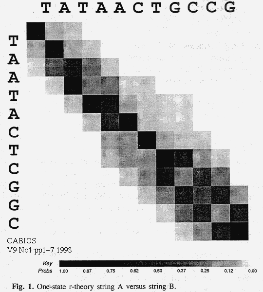
The r-theory algorithm can be run in reverse to give D', where D'i+1,j+1 is the message length required to generate A[i+1..|A|] and B[j+1..|B|] in some way. Adding corresponding elements of D and D' gives a (-log2) probability density plot of all alignments, as in figure 1. This density plot shows the limits of certainty to inferences of the alignment and hence the most recent common ancestor of A and B.
The r-theory algorithm for multi-state models is obtained by similar modifications to Gotoh's algorithm.

Experiments were done to test the ability of different alignment methods to recover the parameters of a known, artificial, evolutionary process. Strings were generated by computer according to known models with known parameter values. Attempts were then made to infer those parameter values by different methods. A good method should be able to recover the true values with reasonable accuracy under such ideal conditions.
In the first set of experiments, a 1-state generation-machine was used to generate pairs of strings. The parameter settings of the machine were varied systematically. For each setting, ten pairs of strings were generated. The string length was 1500. The observed proportions of the various instructions were recorded for each pair and their means and standard-deviations were calculated for each setting. Message lengths based on the "true" alignments were also calculated.
In total, four ways of estimating the machine parameters were tried, all based on the 1-state model: (i) Instruction probabilities were estimated from instruction frequencies in an optimal alignment which was obtained by the iterative process described in section 2. In a cheat, the true machine parameters were used as the initial parameter estimates for the process. This starting point would be unknown in reality but its use was expected to avoid the problem of getting trapped in local minima at high levels of mutation - as turned out to be the case. Its use could be simulated by a systematic and slow search through the parameter space. (ii) As for (i) but arbitrary initial parameter estimates were used. (iii) As for (i) (cheat) except that the r-theory algorithm was used, averaging over all alignments. (iv) As for (iii) but arbitrary initial parameter estimates were used. The means and standard deviations of the parameter values estimated in each of the four ways were calculated.
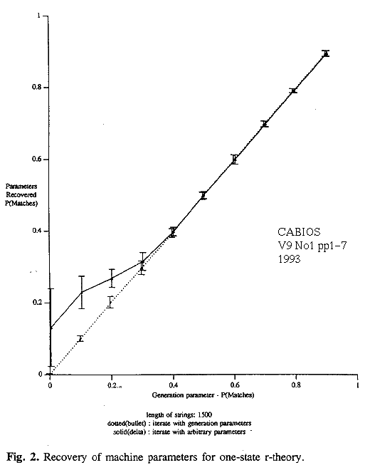
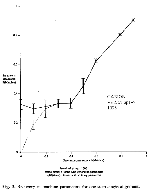
Selected results of the experiments on the 1-state model are collected in table 1, which gives the actual and inferred parameters, and in figures 2 and 3. They show that all methods perform well for small amounts of mutation but that there are deviations for less similar strings.
The r-theory gives good results. If starting from arbitrary initial estimates, it may become trapped in local-minima at very high levels of mutation, when P(match) falls below 0.4. However the true values can be detected as such if they are encountered; a systematic search, or the cheat, finds them right down to P(match)~0 (figure 2, dotted line). The search-space must be very "flat" for strings of such marginal similarity because the message lengths differ very little (but in the right way) for quite different parameter estimates.
A single optimal alignment gives biased results, consistently over-estimating P(match) when P(match) is above 0.6. As P(match) falls below 0.5 the single alignment tends to favour the main diagonal of the D matrix, giving estimated values close to the chance figure for DNA, 0.25 (figure 3). Interestingly, as the true value of P(match) falls near to 0.0, the strings are increasingly related in a negative way and the estimates by this method improve again, given a good starting point.
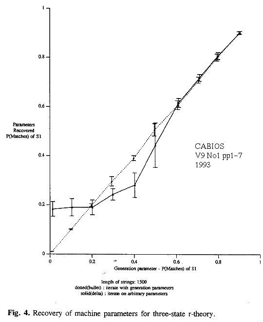
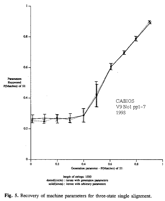
Similar experiments were performed on the 3-state model. The parameters of the machine were varied in a systematic way. Ten pairs of strings were generated for each parameter setting. The string length was 1500. As above, four ways of attempting to recover the parameters, given the strings, were tried. These were all based on the 3-state model and involved (i) an optimal alignment starting from the true parameter values (cheat), (ii) an optimal alignment starting from arbitrary initial values, (iii) r-theory starting from true parameter values (cheat) and (iv) r-theory starting from arbitrary initial values. Selected results are given in table 2 and in figures 4 and 5.
The r-theory gives good estimates. It is likely to get caught in a local minimum, if started from arbitrary initial parameter estimates, for P(match|S1)<0.5. However, if the true parameters values are found they can be detected as such down to P(match|S1)~0 (figure 4).
Inferences based on an optimal alignment underestimate the probability of indels in S1 and overestimate the probability of changes for similar strings. Parameter estimates for states S2 and S3 are poor. Results are of little value when P(match|S1)<0.5 (figure 5).
Experiments were not performed on the 5-state model due to the large number of degrees of freedom that it has and because of the amount of computer time required.
Experiments indicate that the r-theory, based on all alignments, can be used to recover accurate, unbiased estimates of the parameters of the evolutionary process that gave rise to two strings A and B. This is assuming that the true model is known apriori, but that its parameters are not. Previous work[Alli2] indicate that the true model can also be inferred, given enough data. Our probabilistic finite-state machines can approximate many models and are implicit in many alignment algorithms. A probability density plot derived from the r-theory, as in figure 1, indicates the probabilities of possible alignments and thus of possible common ancestors of A and B. The ancestor cannot be assumed to lie on an optimal alignment.
In contrast, parameter estimates based on a single optimal alignment are biased. For example in the 1-state model, P(match) is overestimated when the true value is greater than 0.6 and the estimate is of no value when the true value is less than 0.5. The reason is easy to see: evolution is a random process and the probability that it follows the optimum path is small!
The r-theory programs based on 1, 3 and 5-state models are written in C and are available, free for non-profit, non-classified teaching and research purposes, by email (only) from: http://www.csse.monash.edu.au/~lloyd/tildeStrings/. At least a good work-station with floating-point hardware is required for their use.
|
More recent work on alignment,
can be found at
~lloyd/tildeStrings/
including
fast algorithms,
multiple alignment,
DNA modelling & compression,
alignment of medium to low information content strings. |
Received on December 10, 1991; accepted on June 2, 1992.
    :PM=0.794(0.005) PC=0.145(0.007) PID=0.061(0.006) ML=4965.4(40.83) B/S=1.655(0.014)
opt1:PM=0.803(0.005) PC=0.147(0.007) PID=0.050(0.006) ML=4868.3(44.06) B/S=1.623(0.015)
opt2:PM=0.801(0.005) PC=0.151(0.005) PID=0.047(0.004) ML=4868.0(44.05) B/S=1.623(0.015)
rth1:PM=0.793(0.006) PC=0.145(0.005) PID=0.062(0.007) ML=4799.1(35.13) B/S=1.600(0.012)
rth2:PM=0.793(0.006) PC=0.145(0.005) PID=0.062(0.007) ML=4799.1(35.09) B/S=1.600(0.012)
---------------------------------------------------------------------------------------
    :PM=0.601(0.009) PC=0.279(0.006) PID=0.120(0.010) ML=6208.7(77.93) B/S=2.070(0.026)
opt1:PM=0.624(0.014) PC=0.315(0.019) PID=0.061(0.010) ML=5815.7(65.89) B/S=1.939(0.022)
opt2:PM=0.624(0.014) PC=0.315(0.019) PID=0.061(0.010) ML=5815.7(65.89) B/S=1.939(0.022)
rth1:PM=0.601(0.013) PC=0.276(0.011) PID=0.123(0.017) ML=5624.7(40.19) B/S=1.875(0.013)
rth2:PM=0.601(0.013) PC=0.278(0.011) PID=0.121(0.018) ML=5624.7(40.21) B/S=1.875(0.013)
---------------------------------------------------------------------------------------
    :PM=0.399(0.008) PC=0.419(0.010) PID=0.182(0.007) ML=7187.2(42.71) B/S=2.396(0.014)
opt1:PM=0.334(0.036) PC=0.656(0.042) PID=0.010(0.007) ML=6086.8(42.76) B/S=2.029(0.014)
opt2:PM=0.334(0.036) PC=0.656(0.042) PID=0.010(0.007) ML=6086.8(42.76) B/S=2.029(0.014)
rth1:PM=0.395(0.012) PC=0.422(0.015) PID=0.183(0.008) ML=5991.2( 9.93) B/S=1.997(0.003)
rth2:PM=0.399(0.012) PC=0.439(0.018) PID=0.162(0.015) ML=5991.1(10.02) B/S=1.997(0.003)
---------------------------------------------------------------------------------------
    :PM=0.198(0.010) PC=0.559(0.012) PID=0.243(0.010) ML=7788.6(56.24) B/S=2.596(0.019)
opt1:PM=0.296(0.061) PC=0.693(0.070) PID=0.012(0.011) ML=6118.5(83.02) B/S=2.040(0.028)
opt2:PM=0.311(0.044) PC=0.677(0.054) PID=0.012(0.011) ML=6119.4(82.72) B/S=2.040(0.028)
rth1:PM=0.202(0.016) PC=0.555(0.018) PID=0.243(0.011) ML=6035.6( 1.76) B/S=2.012(0.001)
rth2:PM=0.268(0.025) PC=0.536(0.023) PID=0.196(0.016) ML=6036.3( 2.33) B/S=2.012(0.001)
---------------------------------------------------------------------------------------
    :PM=0.100(0.007) PC=0.628(0.010) PID=0.272(0.010) ML=7874.1(53.21) B/S=2.625(0.018)
opt1:PM=0.187(0.032) PC=0.804(0.025) PID=0.009(0.007) ML=6093.3(60.02) B/S=2.031(0.020)
opt2:PM=0.296(0.035) PC=0.695(0.042) PID=0.009(0.007) ML=6102.6(65.93) B/S=2.034(0.022)
rth1:PM=0.101(0.008) PC=0.628(0.011) PID=0.272(0.010) ML=6031.7( 3.04) B/S=2.011(0.001)
rth2:PM=0.229(0.045) PC=0.572(0.047) PID=0.198(0.013) ML=6035.8( 3.26) B/S=2.012(0.001)
---------------------------------------------------------------------------------------


PM=P(match), PC=P(change), PID=P(indel),
ML Message Length, B/S bits per symbol

(i)       : true generation parameters
(ii)  opt1: single optimal alignment, true initial parameters
(iii) opt2: single optimal alignment, arbitrary initial parameters
(iv)  rth1: r-theory, true initial parameters
(v)   rth2: r-theory, arbitrary initial parameters

Table 1: Results for 1-State Model.


    : ML=6784.3(73.84) B/S=2.261(0.025)
      S1 0.608(0.013) 0.237(0.014) 0.078(0.004) 0.078(0.004)
      S2 0.252(0.016) 0.098(0.012) 0.593(0.025) 0.057(0.011)
opt1: ML=6077.6(40.75) B/S=2.026(0.014)
      S1 0.607(0.021) 0.306(0.033) 0.044(0.006) 0.044(0.006)
      S2 0.447(0.034) 0.004(0.001) 0.545(0.035) 0.004(0.001)
opt2: ML=6078.0(40.87) B/S=2.026(0.014)
      S1 0.607(0.021) 0.306(0.033) 0.044(0.006) 0.044(0.006)
      S2 0.449(0.033) 0.004(0.001) 0.543(0.034) 0.004(0.001)
rth1: ML=5813.6(37.31) B/S=1.938(0.012)
      S1 0.608(0.018) 0.231(0.030) 0.081(0.009) 0.081(0.009)
      S2 0.253(0.020) 0.099(0.008) 0.596(0.024) 0.053(0.007)
rth2: ML=5815.6(37.38) B/S=1.939(0.012)
      S1 0.617(0.018) 0.191(0.038) 0.096(0.015) 0.096(0.015)
      S2 0.199(0.039) 0.095(0.022) 0.551(0.029) 0.155(0.024)
-------------------------------------------------------------
    : ML=7701.3(65.00) B/S=2.567(0.022)
      S1 0.400(0.012) 0.363(0.010) 0.118(0.006) 0.118(0.006)
      S2 0.244(0.015) 0.101(0.013) 0.601(0.026) 0.054(0.007)
opt1: ML=6113.4(92.67) B/S=2.038(0.031)
      S1 0.288(0.043) 0.702(0.057) 0.005(0.007) 0.005(0.007)
      S2 0.220(0.196) 0.082(0.111) 0.651(0.222) 0.047(0.054)
opt2: ML=6099.3(92.16) B/S=2.033(0.031)
      S1 0.288(0.045) 0.703(0.058) 0.005(0.007) 0.005(0.007)
      S2 0.182(0.193) 0.082(0.111) 0.689(0.234) 0.047(0.054)
rth1: ML=6030.7(7.82) B/S=2.010(0.003)
      S1 0.391(0.010) 0.373(0.008) 0.118(0.007) 0.118(0.007)
      S2 0.252(0.025) 0.108(0.010) 0.583(0.037) 0.057(0.009)
rth2: ML=6033.6(9.21) B/S=2.011(0.003)
      S1 0.281(0.050) 0.259(0.028) 0.230(0.011) 0.230(0.011)
      S2 0.258(0.029) 0.257(0.024) 0.233(0.016) 0.253(0.010)
-------------------------------------------------------------

(i)       : true generation parameters
(ii)  opt1: 1 optimal alignment, true initial parameters
(iii) opt2: 1 optimal alignment, arbitrary initial parameters
(iv)  rth1: r-theory, true initial parameters
(v)   rth2: r-theory, arbitrary initial parameters

S1 is copy and change state
   P(copy|S1) P(change|S1) P(insert|S1)=P(delete|S1)
S2 is insertA state
   P(copy|S2) P(change|S2) P(insert|S2) P(delete|S2)
S3 is insertB state, similar to S2

Table 2: Results for 3-State Model.
`Computer Applications in the BioScience' (CABIOS) became `The Journal of Bioinformatics' c1999. [V9(No1)]
L. Allison, School of Computer Science and Software Engineering, Monash University, Australia 3168. Created with "vi (Linux + IRIX)", charset=iso-8859-1