Appears in: Seventh Pacific Rim International Conference on Artificial Intelligence (PRICAI-2002), Tokyo, Japan, 18-22 August 2002.
Leigh J. Fitzgibbon, David L. Dowe, and Lloyd Allison
{leighf,dld,lloyd}@bruce.csse.monash.edu.au
This paper investigates the coding of change-points in the information-theoretic Minimum Message Length (MML) framework. Change-point coding regions affect model selection and parameter estimation in problems such as time series segmentation and decision trees. The Minimum Message Length (MML) and Minimum Description Length (MDL78) approaches to change-point problems have been shown to perform well by several authors. In this paper we compare some published MML and MDL78 methods and introduce some new MML approximations called `MMLDc' and `MMLDF'. These new approximations are empirically compared with Strict MML (SMML), Fairly Strict MML (FSMML), MML68, the Minimum Expected Kullback-Leibler Distance (MEKLD) loss function and MDL78 on a tractable binomial change-point problem.
Change-points can be found in many machine learning problems. They arise where there is a need to partition data into contiguous groups which are to be modelled distinctly. The inference of change-points (the boundaries of the contiguous groups) is important since change-points describe a point of transition between different states of stochastic behaviour of the data. They can be used to explain the generating process and also for prediction of future data.
The Minimum Message Length (MML) principle [1,2,3] is an invariant Bayesian point estimation technique based on information theory.
MML selects regions from the parameter space which contain models that can justify themselves with high posterior probability mass [3, page 276].
Using MML we are able to capture the important information in the posterior. For example, the best explanation of the data might be that ``a change-point occurred between times ![]() and
and ![]() and the point estimate that best summarizes this region is
and the point estimate that best summarizes this region is ![]() ''. The MML method is especially useful when many change-points are being estimated and on large data-sets - for example, segmentation of a DNA string. DNA strings can be very large, containing millions of characters. It would be impractical to deal with a posterior distribution over such strings using contemporary computational techniques.
''. The MML method is especially useful when many change-points are being estimated and on large data-sets - for example, segmentation of a DNA string. DNA strings can be very large, containing millions of characters. It would be impractical to deal with a posterior distribution over such strings using contemporary computational techniques.
Previous work on coding change-point parameters in the MML framework has resulted in analytical approximations which treat the change-point as a continuous parameter [4,5,6,7] or avoid stating them altogether [8]. These methods work well in practice. However, change-points are realized as discrete parameters since they partition a data sample, and in this paper we investigate new MML approximations which treat them discretely.
The paper proceeds by describing a binomial change-point problem. We then consider the two computationally infeasible MML criteria: Strict MML (SMML) and Fairly Strict MML (FSMML) in Section 3.1 and 3.2. The algorithms to compute the SMML and FSMML codes have exponential time complexity for the binomial problem, which limits the experiments to small samples, but the results still give insight into the behaviour of the methods. We then describe two new approximations called MMLDc and MMLDF. These are practical methods that are motivated by SMML (in part), FSMML and MML87 [2]. In Section 5 we empirically compare these new approximations with SMML, FSMML and other existing methods.
A Bernoulli trial is conducted with ![]() independent coin tosses. The results are recorded in a binary string
independent coin tosses. The results are recorded in a binary string ![]() , where
, where ![]() and
and ![]() . It is suspected that the bias of the coin may have changed at some point in time,
. It is suspected that the bias of the coin may have changed at some point in time, ![]() , during the trial. Given the data from the trial, we wish to infer the best explanation: was there a change-point and, if so, where was it? We denote the change-point parameter by
, during the trial. Given the data from the trial, we wish to infer the best explanation: was there a change-point and, if so, where was it? We denote the change-point parameter by ![]() and its parameter-space by
and its parameter-space by ![]() . We often speak in terms of the number of groups of data rather than the number of change-points. And, in our notation, we use
. We often speak in terms of the number of groups of data rather than the number of change-points. And, in our notation, we use ![]() for the number of groups (
for the number of groups (![]() ).
).
The likelihood for the change-point model is:
 |
(1) |
The likelihood function for an ordered Bernoulli trial, which we will be using for ![]() ,
, ![]() and
and ![]() is:
is:
| (2) |
To make the SMML and FSMML solutions computationally feasible, the experiments are simplified as follows. For ![]() , we use a uniform prior over the change-point location (i.e.
, we use a uniform prior over the change-point location (i.e.
![]() ), and we have a uniform prior for the number of change-points (i.e. h(G=1) = h(G=2) = 0.5). The
), and we have a uniform prior for the number of change-points (i.e. h(G=1) = h(G=2) = 0.5). The ![]() ,
, ![]() and
and ![]() likelihood functions that we have chosen to use have fixed biases, and therefore have no free parameters. The biases we use are 0.25, 0.15 and 0.75 for
likelihood functions that we have chosen to use have fixed biases, and therefore have no free parameters. The biases we use are 0.25, 0.15 and 0.75 for ![]() ,
, ![]() and
and ![]() respectively. We use fixed coins to reduce the estimation problem to the two discrete parameters of interest:
respectively. We use fixed coins to reduce the estimation problem to the two discrete parameters of interest: ![]() and
and ![]() . This is necessary to make the construction of the SMML and FSMML (code-books and) estimators feasible. However, even though we are using such a simple model there is still an exponential step (see Section 3.1), so experimenting with large amounts of data is not possible.
. This is necessary to make the construction of the SMML and FSMML (code-books and) estimators feasible. However, even though we are using such a simple model there is still an exponential step (see Section 3.1), so experimenting with large amounts of data is not possible.
In the Minimum Message Length (MML) framework [1,2,3], inference is framed as a coding process. The aim is to construct a code-book that would (hypothetically) allow for the transmission of the data in a two-part message over a noiseless channel as briefly as possible. From coding theory we know that an event with probability ![]() can be encoded in a message with length
can be encoded in a message with length
![]() bits using an ideal Shannon code. Using a Bayesian setting, the sender and receiver agree on a prior distribution
bits using an ideal Shannon code. Using a Bayesian setting, the sender and receiver agree on a prior distribution ![]() and likelihood function
and likelihood function
![]() over the parameter space
over the parameter space ![]() and data-space
and data-space ![]() . An estimator is a function from the data-space to the parameter-space, denoted
. An estimator is a function from the data-space to the parameter-space, denoted
![]() . After observing some data
. After observing some data ![]() , we can use an estimator to construct a two-part message encoding the estimate
, we can use an estimator to construct a two-part message encoding the estimate
![]() in the first part and then the data using the estimate,
in the first part and then the data using the estimate, ![]() , in the second.
, in the second.
The probability that ![]() returns an estimate
returns an estimate
![]() is
is
![]() , where
, where ![]() is the marginal probability of the data,
is the marginal probability of the data, ![]() . The length of the first part of the message is therefore
. The length of the first part of the message is therefore
![]() , and the length of the second part of the message is
, and the length of the second part of the message is
![]() . The sender and receiver will use the code-book with estimator,
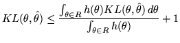
. The sender and receiver will use the code-book with estimator, ![]() , which minimises the expected message length:
, which minimises the expected message length:
The estimator which minimises ![]() is called the Strict Minimum Message Length (SMML) estimator [2, page 242] [9,10,3]. The construction of
is called the Strict Minimum Message Length (SMML) estimator [2, page 242] [9,10,3]. The construction of ![]() is NP-hard for most distributions. The only distributions that it has reportedly been constructed for are the binomial and trinomial (trinomial using a heuristic) [9] and
is NP-hard for most distributions. The only distributions that it has reportedly been constructed for are the binomial and trinomial (trinomial using a heuristic) [9] and ![]() [11, page 22].
[11, page 22].
The construction of SMML estimators is simplified when there exists a sufficient statistic of lesser dimension than the data-space. Unfortunately, for univariate change-point parameters, the minimal sufficient statistics are of the same dimension as the data. Since we therefore cannot reduce the dimensionality of the data-space, we are left with the SMML code-book construction problem of trying to optimally assign the ![]() elements of the data-space to estimates. For the experiments in this paper we use an EM algorithm which randomly selects an element of the data-space and then finds the optimal code-book assignment
elements of the data-space to estimates. For the experiments in this paper we use an EM algorithm which randomly selects an element of the data-space and then finds the optimal code-book assignment
![]() using:
using:
![]() .
.
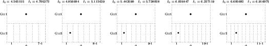
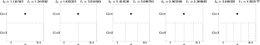
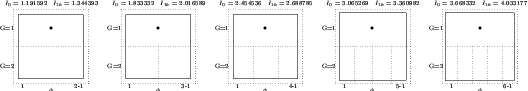
This is not guaranteed to minimise ![]() since the algorithm can easily get stuck in local optima. To try and avoid this, we iterate the SMML algorithm a number of times with and without seeding the algorithm with the FSMML partition discussed in the next section. The resulting algorithm still has exponential time complexity. The SMML estimates for up to
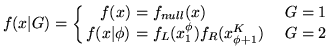
since the algorithm can easily get stuck in local optima. To try and avoid this, we iterate the SMML algorithm a number of times with and without seeding the algorithm with the FSMML partition discussed in the next section. The resulting algorithm still has exponential time complexity. The SMML estimates for up to ![]() can be seen in Figure 1. The bold dots in the diagram illustrate the point estimates that are used in the code-book. We can see that for up to, and including,
can be seen in Figure 1. The bold dots in the diagram illustrate the point estimates that are used in the code-book. We can see that for up to, and including, ![]() the estimator always infers that there was no change-point. As the data-space gets larger, point estimates start appearing to the left of the change-point parameter space. This asymmetry is explained by the choice of biases used.
the estimator always infers that there was no change-point. As the data-space gets larger, point estimates start appearing to the left of the change-point parameter space. This asymmetry is explained by the choice of biases used.
The FSMML [12] estimator is an approximation to SMML based on a partition of the parameter space. The FSMML expected message length is:
We minimise ![]() by searching for the optimal partition of the parameter-space and the
by searching for the optimal partition of the parameter-space and the
![]() for each segment of the partition. Since
for each segment of the partition. Since ![]() consists of a sum over independent partitions, we can use W. D. Fisher's [13] polynomial time dynamic programming algorithm
consists of a sum over independent partitions, we can use W. D. Fisher's [13] polynomial time dynamic programming algorithm![[*]](footnote.png) . We therefore seek the partition of change-points and the estimates which minimise
. We therefore seek the partition of change-points and the estimates which minimise ![]() . We allow the partition to contain models from different subspaces since all we are attempting to do is group similar models in such a way that minimises the expected two-part message length.
. We allow the partition to contain models from different subspaces since all we are attempting to do is group similar models in such a way that minimises the expected two-part message length.
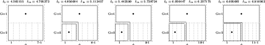
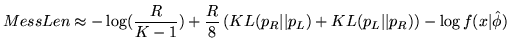
The algorithm we use is guaranteed to find the optimal solution. It consists of a high-order polynomial step to find the partition (using Fisher's algorithm), and an exponential step to compute a revised version of the message length (![]() in the Figures). The FSMML partitions for up to
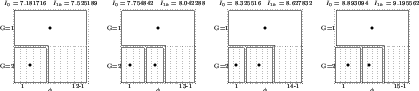
in the Figures). The FSMML partitions for up to ![]() can be seen in Figure 2. The partition is represented by the solid shapes, and the bold dots represent the point estimates used in each region. We can see that once
can be seen in Figure 2. The partition is represented by the solid shapes, and the bold dots represent the point estimates used in each region. We can see that once ![]() is greater than eight, the partitions consist of models from different subspaces. This allows data generated by change-points on the right to be modelled by the no change-point model. What the FSMML partition is saying is that we cannot reliably distinguish between models in this region, and they are best modelled with the no change-point model. In the figures, the FSMML code-book looks very similar to the SMML code-book. However, as expected, for many values of
is greater than eight, the partitions consist of models from different subspaces. This allows data generated by change-points on the right to be modelled by the no change-point model. What the FSMML partition is saying is that we cannot reliably distinguish between models in this region, and they are best modelled with the no change-point model. In the figures, the FSMML code-book looks very similar to the SMML code-book. However, as expected, for many values of ![]() , the SMML estimator has a slightly better message length. This is because it is able to individually assign elements of the data-space to estimates.
, the SMML estimator has a slightly better message length. This is because it is able to individually assign elements of the data-space to estimates.
Oliver, Baxter and co-workers have applied the MML68 [1] estimator methodology to the segmentation problem with Gaussian segments [4] [11, chapter 9] [5,6]. They have derived MML formulas for stating the change-point locations to an optimal precision independently of the segment parameters. The same method has been used [7] for the problem of finding change-points in noisy binary sequences [14] - where it compared favourably with Akaike's Information Criterion (AIC), Schwarz's Bayesian Information Criterion (BIC), an MDL-motivated metric of Kearns et al. [14] and a more correct version of Minimum Description Length[7].
We apply the MML68 approximation to the binomial problem in this paper. Assuming that the true change-point is uniformly distributed in some range of width, ![]() , we encode the data using the point estimate
, we encode the data using the point estimate
![]() at the centre of this region. The true change-point is equally likely to be to the right or to the left of the point estimate. If it is located to the right then its expected value is
at the centre of this region. The true change-point is equally likely to be to the right or to the left of the point estimate. If it is located to the right then its expected value is
![]() , and if it is located to the left its expected value is
, and if it is located to the left its expected value is
![]() . The expected message length is computed by averaging the expected coding inefficiency of these two scenarios which for our Bernoulli problem simplifies to an expression involving the Kullback-Leibler distance,
. The expected message length is computed by averaging the expected coding inefficiency of these two scenarios which for our Bernoulli problem simplifies to an expression involving the Kullback-Leibler distance, ![]() :
:
Minimum Message Length approximation D (MMLD) can be thought of as a numerical approximation to FSMML. It was proposed by D. L. Dowe and has been investigated by his student [15]. MMLD is based on choosing a region ![]() of the parameter space after observing some data. It was partly motivated by improving the Taylor expansion approximation of MML87 [2] while retaining invariance and, like MML87, avoids the problem of creating the whole code-book, which would typically require enumeration of the data and parameter spaces in SMML and FSMML. Given an uncertainty region,
of the parameter space after observing some data. It was partly motivated by improving the Taylor expansion approximation of MML87 [2] while retaining invariance and, like MML87, avoids the problem of creating the whole code-book, which would typically require enumeration of the data and parameter spaces in SMML and FSMML. Given an uncertainty region, ![]() , MMLD approximates the length of the first part of the message as the negative log integral of the prior over
, MMLD approximates the length of the first part of the message as the negative log integral of the prior over ![]() (like FSMML). The length of the second part is approximated by the expected value (with respect to the prior), over
(like FSMML). The length of the second part is approximated by the expected value (with respect to the prior), over ![]() , of the negative log-likelihood. This gives rise to an MMLD message length of
, of the negative log-likelihood. This gives rise to an MMLD message length of
Equation 6 makes no explicit claim about which point estimate should be used to encode data for the region, ![]() . Once the region has been found which minimises it, we need to find a point estimate which summarizes the models in the region. Since the estimates produced by the FSMML estimator are equivalent to the minimum expected Kullback-Leibler distance estimator (the expectation being taken with respect to the prior over the region, rather than the posterior) [12,10], we have used this for the experiments involving MMLD:
. Once the region has been found which minimises it, we need to find a point estimate which summarizes the models in the region. Since the estimates produced by the FSMML estimator are equivalent to the minimum expected Kullback-Leibler distance estimator (the expectation being taken with respect to the prior over the region, rather than the posterior) [12,10], we have used this for the experiments involving MMLD:
Whereas FSMML can build code-books consisting of non-contiguous regions (i.e., combine modes or models from different subspaces) with minimum expected message length, MMLD cannot in general. This is because MMLD does not take into account the similarity of the models it combines in ![]() - it only cares about their prior probability and likelihood. If we attempt to build non-contiguous regions, then in variable dimension problems or where the likelihood is multi-modal, MMLD will possibly combine modes. The models contained within these modes may be quite different (i.e., have large Kullback-Leibler distances), or they may be similar (i.e., have small Kullback-Leibler distances). For the latter case, combining modes is a valid thing to do. However, in general, we would expect the models contained in two distinct modes to be quite different and, for inference, we risk underestimating the message length if they are grouped into the same region.
- it only cares about their prior probability and likelihood. If we attempt to build non-contiguous regions, then in variable dimension problems or where the likelihood is multi-modal, MMLD will possibly combine modes. The models contained within these modes may be quite different (i.e., have large Kullback-Leibler distances), or they may be similar (i.e., have small Kullback-Leibler distances). For the latter case, combining modes is a valid thing to do. However, in general, we would expect the models contained in two distinct modes to be quite different and, for inference, we risk underestimating the message length if they are grouped into the same region.
So, rather than simply choose the region ![]() to optimise Dowe's MMLD message length expression in Equation 6, Fitzgibbon has suggested that we invoke the FSMML `Boundary Rule' [12] to determine whether a model should be considered for membership of
to optimise Dowe's MMLD message length expression in Equation 6, Fitzgibbon has suggested that we invoke the FSMML `Boundary Rule' [12] to determine whether a model should be considered for membership of ![]() . The Boundary Rule is a heuristic used to choose the optimal partition for the FSMML expected message length equation (Equation 4), where a candidate model
. The Boundary Rule is a heuristic used to choose the optimal partition for the FSMML expected message length equation (Equation 4), where a candidate model ![]() is considered to be a member of the region (with point estimate
is considered to be a member of the region (with point estimate
![]() - the minimum prior-weighted expected Kullback-Leibler distance estimate for the region) if the following constraint is satisfied:
- the minimum prior-weighted expected Kullback-Leibler distance estimate for the region) if the following constraint is satisfied:
We denote the MMLD approximation augmented by the FSMML Boundary Rule as MMLDF. While other (non-contiguous) versions of MMLD exist, throughout the remainder of this paper, MMLDc will refer to using a contiguous region (i.e. ![]() contains only models of the same dimension and from a single mode). We include both MMLDc and MMLDF in the experiments to compare the advantage of allowing the region to consist of models from different subspaces. For the binomial problem with known biases, the parameter space is discrete - so an exhaustive search for the optimal region was performed.
contains only models of the same dimension and from a single mode). We include both MMLDc and MMLDF in the experiments to compare the advantage of allowing the region to consist of models from different subspaces. For the binomial problem with known biases, the parameter space is discrete - so an exhaustive search for the optimal region was performed.
Compact coding methods attempt to minimise the expected length of a two-part message. However, they cannot be judged on this criterion since - other than SMML and FSMML - the methods only approximate the message length. Furthermore, we are not really interested in creating short messages per se but rather in how good the inferred statistical model is. The definition of a good model will depend on what use the model will be put to. We therefore use the following general criteria: the Kullback-Leibler (KL) distance between the true and inferred models; and the mean squared error in estimation of the change-point location (if it exists). We have compared the MMLD approximation both with and without the FSMML Boundary Rule (MMLDF and MMLDc respectively) with SMML, FSMML, MML68 (as described in Section 3.3), Minimum Description Length (MDL78) [16] and the Minimum Expected KL Distance loss function (MEKLD) [10]. We ran ![]() trials for each
trials for each ![]() where we sampled from the prior and then generated data. Each method was given the data and the biases of the coins used to generate the data and then asked to infer whether or not a change-point occurred and, if so, where it was located.
where we sampled from the prior and then generated data. Each method was given the data and the biases of the coins used to generate the data and then asked to infer whether or not a change-point occurred and, if so, where it was located.
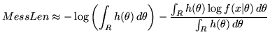
We have plotted the average KL distance for each method in Figure 3. The SMML and FSMML estimators had significantly higher KL distances than the other methods for ![]() . MEKLD had the lowest on average, as expected. MML68 performed well and was not far behind MEKLD. Our MMLDF estimator was close behind MML68 and slightly better than our MMLDc estimator.
. MEKLD had the lowest on average, as expected. MML68 performed well and was not far behind MEKLD. Our MMLDF estimator was close behind MML68 and slightly better than our MMLDc estimator.
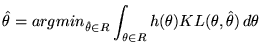
Figure 4 shows the average squared error in estimating the change-point location for each method. The average is taken over the instances where the method correctly inferred that there was a change-point. The SMML and FSMML estimators performed exceptionally well. Their good performance here and poor KL distance performance indicates that they prefer not to infer a change-point unless they are reasonably certain of its location. The MMLDF estimator comes second to SMML and FSMML for ![]() . The MML68 method, which had very good KL distance performance, performed poorly for this criterion.
. The MML68 method, which had very good KL distance performance, performed poorly for this criterion.
We note that MMLDF outperforms MMLDc for both criteria, therefore providing evidence that building non-contiguous coding regions - which SMML theory and FSMML theory both advocate - is advantageous. The MMLDF estimator appears to be robust and has good explanatory (i.e., has small squared error in change-point location when correctly inferring change-points) and predictive powers (i.e., has small KL distances).
We have empirically compared a number of information-theoretic methods for estimating change-points including two new Minimum Message Length approximations. The comparison was based on a binomial problem using small sample sizes which allowed us to include the computationally impractical Strict MML (SMML) and Fairly SMML (FSMML) estimators. In the comparison we found that the performance of the MMLDc approximation was improved by incorporating the Kullback-Leibler Boundary Rule, therefore allowing coding regions to contain models from different subspaces (MMLDF) whilst still approximating an efficient FSMML code-book. MMLDF was robust and performed well in terms of Kullback-Leibler distance and (squared) error in estimation of the change-point location (where inferred). Use of MMLD and variations for more difficult problems will be investigated in forthcoming work.
This document was generated using the LaTeX2HTML translator Version 2K.1beta (1.57)
Copyright © 1993, 1994, 1995, 1996,
Nikos Drakos,
Computer Based Learning Unit, University of Leeds.
Copyright © 1997, 1998, 1999,
Ross Moore,
Mathematics Department, Macquarie University, Sydney.
The command line arguments were:
latex2html -local_icons -notransparent -white -antialias -nonavigation -split 0 pricai
The translation was initiated by Leigh Fitzgibbon on 2002-05-27
![\includegraphics[width=300pt]{/home/leighf/static/Paper-PRICAI2002/res1}](img73.png)
![\includegraphics[width=300pt]{/home/leighf/static/Paper-PRICAI2002/res2}](img74.png)