MODEL SET UP
The model is a horizontal plane at a fixed lithostatic pressure (p), fluid absent and is deformed in pure shear with a horizontal shortening axis. The bulk modulus, K, and shear modulus G are such that they yield a Poisson ratio n
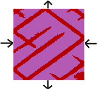
Figure 1. Model 17: study of stress distribution in a layered system, the embedded layer in the middle has elastic moduli (Shear and Bulk Moduli) an order of magnitude higher than surroudings.
A) State step 75000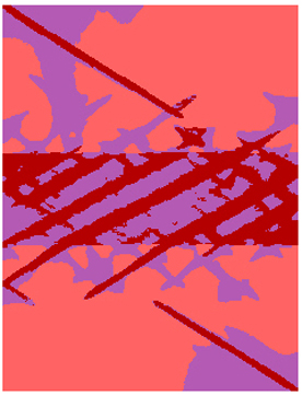
|
B) Mean stress
distribution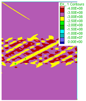
|
C)
Mean stress profile (zoom in a 400m profile) 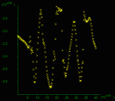
|
Figure 2. Model 18: study of stress distribution in a layered system, the embedded layer in the middle has elastic moduli (Shear and Bulk Moduli) an order of magnitude lower than surroudings.
A) State step 75000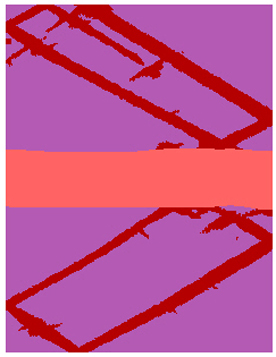
|
B) Mean stress
distribution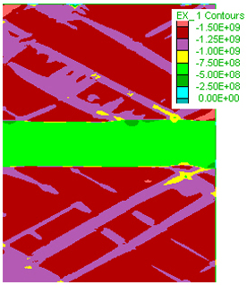
|
C)
Mean stress profile (zoom in a 400m profile) 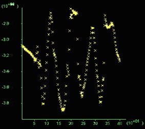 |
Figure 3. Model 20. Like Figure 2 but pore fluids are initially at twice hydrostatic pressure. Step 55000. A) State. Much narrower and numerous shear bands develop compared to the case with no fluids (Fig. 1). Click on figure for movies. B) Is a zoom of a shear band
in A) and shows the fluid flow vectors indicating flow into the shear bands.
C) Pore pressure distribution showing a minimum in the center of the box.
D) Pore pressure profile showing a variation of 0.12 kbar across the area.
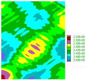
E) Mean stress distribution in a typical area approximately a quarter of the box area. F) Mean stress given in 10^8 Pa (=1 kbar) along a vertical section (x-axis in m), 200 m long through the middle of the box. Note the difference between highs and lows reaches 0.8 kbar and values oscilate around 4 kbar at this stage.
Click on figure to see a movie of the mean stress evolution.
G) Total volume flux vertical profile (in m3), x-axis in 100m.
H) Volume flux profile.
A) State (movie)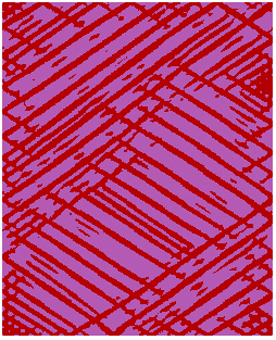
|
B) Zoom of A) plus flow
vectors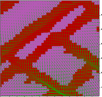
|
C) Pore pressure (movie)
|
D) Pore pressure profile
(movie)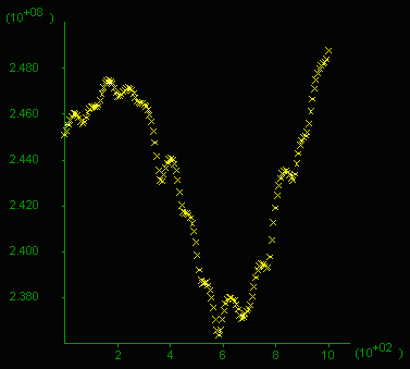
|
E) Mean stess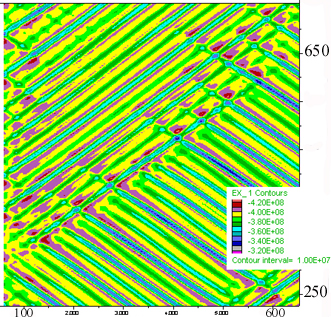
|
F) Mean stress profile
(movie)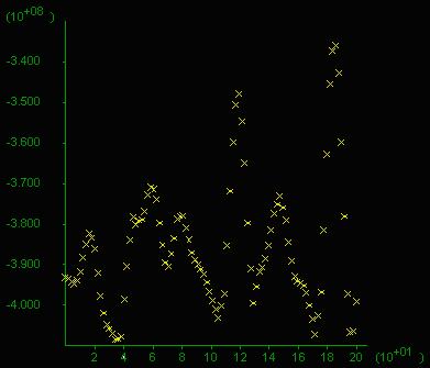
|
G) Volume Flux 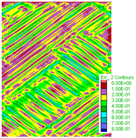
|
H) Volume Flux Profile 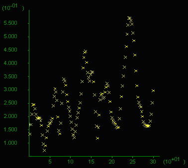
|