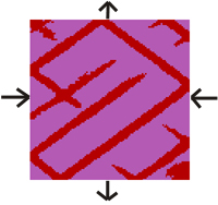
This section illustrates the role of the friction F and dilation angles Y in the development of shear bands during pure shear deformation (non-associated plasticity). It also illustrates the role of grid resolution and the role of the dimensionless parameter B defined by Poliakov et al. (1994) for these models.
Related Pages |
| Strain
incompatibility
during shearing
|
Input file
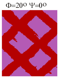
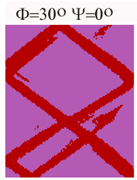
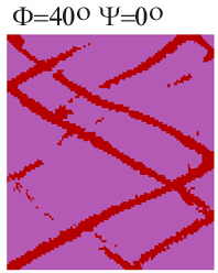
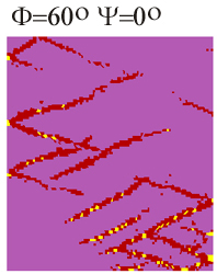
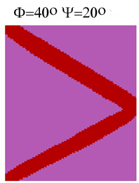
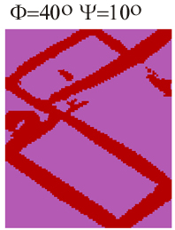
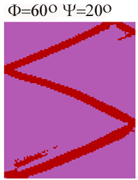
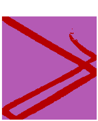
Figure 1. Comparisson between results with different values of friction for dilation of zero and other identical parameters. An increase in the value of the friction angle leads to increased localization of the shear bands and increased irregularity. Note also the change in the angle between the conjugate pair in relation to the horizontal shortening axis. The angle becomes more acute with increasing frictional angle. Remember the acute angle is 2*{45o- (f
 |
 |
 |
 |
 |
 |
|
|
|
|
B) F
|
|
|
Dimensionless parameters is an effective way of simplifying and summarizing the physics of numerical models. The following section is an example of its use.
RW's notes: For calculations using fluids another dimensionless number is necessary which uses the variables related to fluid flow such as permeability and pore pressure gradient. For this, the dimensionless fluid velocity D was created. This is the ratio between the Darcy velocity and the sound velocity:
D= KFLAC* Grad pp / c.
The following models were inspired by and repeat the models described in Poliakov et al. (1994, Fractals, 2, p. 567-581). These authors found that the shear band patterns depend solely on a dimensionless parameter B and the ratio between the size of the mesh and and the system size, L, for a fixed value of the friction angle F
Figure 4 A) Two models with constant B and with the same friction and dilation angles. Pressure and m
The results are different but the style of shear bands developed are similar. The model on the right-hand-side has a fifth of the pressure and shear modulus of the model on the left-hand-side. Because our expectation was to find similar results (Poliakov et al. 1994, Fractal 2), we increased the grid from 100*100, as in the previous models, to 150*150.
The two embedded movies (click on figures) illustrate the evolution of the models as they are strained. In both models the width of the shear bands tend to remain constant throughout, but the number of shear bands decreases with time. Velocity here is half that of the models above.
B) At higher resolution (300*300) the results for the two models converge. Note in the two movies that after the first 30000 to 40000 steps the distribution of shear bands is reasonably stable. Poliakov et al. (1994) concluded, and these calculations confirm, that the non-dimensional parameter B controls the evolution of the system.
M 10, 150*150, T'=12.5,
p=2.e8
Pa, G=5.e9
Pa 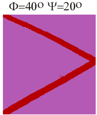 |
M 8, 150*150, T'=2.67,
p=4.e7
Pa, G=1.e9
Pa 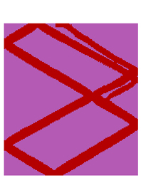 |
M 10b, 300*300, T'=12.5,
p=2.e8
Pa, G=5.e9
Pa 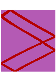 |
M 8b, 300*300, T'=2.67,
p=4.e7
Pa, G=1.e9
Pa 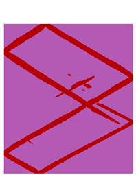
|
Figure 4 (Cont) Different B-values. In c) the value of B is five times smaller than that of D) due to a decrease in the value of the shear modulus G. An important difference is that with the decrease in the value of the shear modulus in D) yielding starts at a much later stage, only after 40000 step at the same deformation velocity (compared with the yilding in C) between 5000 and 10000 steps. This had been predicted by Poliakov et al. (1994) which determined that the time at which the yield limit is reached is proportional to the inverse of G, so five times longer for D) given the same boundary velocity.
| C) M 10b, 300*300, T'=12.5,
p=2.e8
Pa, G=5.e9
Pa |
D) M 15, 300*300, T'=2.67,
p=2.e8
Pa, G=1.e9
Pa 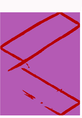
|
Figure 5. Another high resolution model (300*300) was run with even lower lithostatic pressure (1.e7 Pa) and a decrease in T'=1.e7/1.5e7=0.67. B is kept constant by a decrease both the shear and bulk modulus. While in the models in Fig. 4 the role of T' is not visible, the decrease in T' here to a value below unity has lead to the initiation of tensile failure and the emergence of a different pattern.
M 14b, 300*300, T'=0.67,
p=1.e7,
G=0.25e9
Pa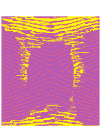 |
Figure 6. Changes in shear band distribution and width as a function of resolution for model 8 above. At 100*100 fewer shear zones developed. At higher resolution the results converge. Poliakov et al. (1994) , using FLAC, found also that . Compare the results here with those in Poliakov et al.'s Fig. 10.
Resolution 100*100 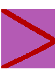
|
Resolution 150*150  |
Resolution 300*300
|
Figure 7. Changes in model 8 as a function of deformation velocity only. Deformation velocity changes the value of B and we should therefore expect some changes in the shear bands. Model on B) was deformed an order of magnitude slower than model on A). Diagram on the right-hand-side shows the history of unbalanced forces as the model develops. When yielding first takes place there is a peak in unbalanced forces which gradually decreases as the model progresses. The histories in both cases are not particularly good.
A) Resolution 150X150  |
History of unbalanced
forces 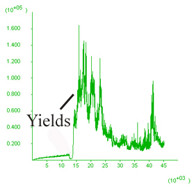 |
B) Resolution 150X150,V/10
 |
History of unbalanced
forces 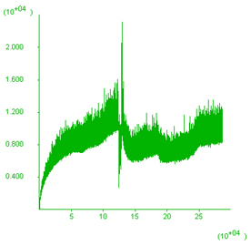 |
| The models illustrate the role played by the friction and dilation angles in the evolution of shear zones during pure shear. This exercise illustrates the use of the dimensionless parameters as an effective way of simplifying and summarizing the physics of numerical models. It illustrates also issues of resolution and that the yielding history is dependent on the amount of straining. |