Workshop 1
23 April 2011
Installing R
The latest version of an R installation binary (or source code) can be downloaded from one of the Comprehensive R Archive Network (or CRAN) mirrors. Having selected one of the (Australian) mirrors, follow one of the sets of instructions below (depending on your operating system).
Windows
- From the list of precompiled binaries, select 'Windows'
- Select the 'base' subdirectory
- Click on 'Download R_2.XX.X for Windows' (where XX.X is the current version number and release).
- Depending on the version of Windows you are running (XP, Vista or Windows 7), run (execute) this downloaded install binary. Note, if you are running Vista, you should execute this binary as Administrator. This ensures that R is installed in the system area (c:\Program Files) rather than in the user space which can lead to issues.
- Under Vista or Windows 7, when warned of either 'unidentified publisher' or 'unknown publisher' respectively, elect to allow or continue
- The installer is fairly straight forward and will guide you through the installation. The default options are typically adequate.
- Startup menus and a desktop icon will be generated

MacOSX
- From the list of precompiled binaries, select 'MacOS X'
- Click on 'R-2.XX.X.pkg' (where XX.X is the current version number and release) to download the installer package. Note, this is for MacOS X 10.5 (Leopard) and 10.6 (Snow Leapard) only. For earlier versions of MacOSX, you will need to scroll down to the link to 'old'
- Run the installer (double click on the image in the new finder window)
- If you are not already logged in as Administrator, you will be prompted for the Administrator password
- The installer is fairly straight forward and will guide you through the installation. The default options are typically adequate.
Linux
- From the list of precompiled binaries, select 'Linux'
- R is available in range of pre-compiled binaries for Debian (Ubuntu), Red Hat and SuSE based distributions
- Quite frankly, if you are a linux user, you do not require instructions!
Basic Syntax
The R environment and command line
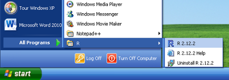
A first look at R
- Double click on the RGui icon on the desktop
- Click the START button from the Windows task bar
- Click Program Files
- Click R2.XX.X (where XX.X is the version and release numbers)
- Click RGui (Gui stands for Graphics User Interface)
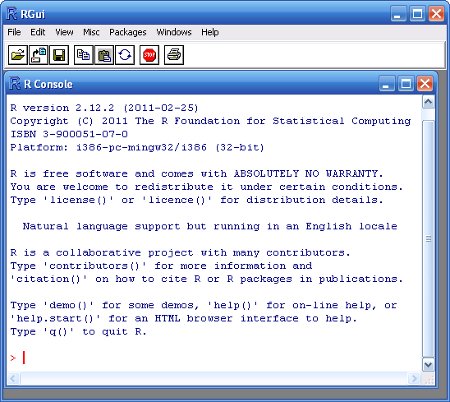
Upon opening R, you are presented with the R Console along with the command prompt (>). R is a command driven application (as opposed to a 'point-and-click' application) and despite the steep learning curve, there are many very good reasons for this.
Commands that you type are evaluated once the Enter key has been pressed
Enter the following command at the command prompt (>);
This evaluates the command five plus one and returns the result (six).. The [1] before the 6 indicates that the object immediately to its right is the first element in the returned object. In this case there is only one object returned. However, when a large set of objects (e.g. numbers) are returned, each row will start with an index number thereby making it easier to count through the elements.
Important definitions
- Object
- As an object oriented language, everything in R is an object. Data, functions even output are objects.
- Vector
- A collection of one or more objects of the same type (e.g. all numbers or all characters).
- Function
- A set of instructions carried out on one or more objects. Functions are typically wrappers for a sequence of instructions that perform specific and common tasks.
- Parameter
- The kind of information passed to a function.
- Argument
- The specific information passed to a function.
- Operator
- A symbol that has a pre-defined meaning. Familiar operators include + - * and /.
Assignment operators <- Assigning a name to an object = Used when defining and specifying function arguments Logical operators (return TRUE or FALSE) Less than Greater than <= Less than or equal >= Greater than or equal == Is the left hand side equal to the right hand side (a query) != Is the left hand side NOT equal to the right hand side (a query) && Are BOTH left hand and right hand conditions TRUE || Are EITHER the left hand OR right hand conditions TRUE
Expressions, Assignment and Arithmetic
Instead of evaluating a statement and printing the result directly to the console, the results of evaluations can be stored in an object via a process called 'Assignment'. Assignment assigns a name to an object and stores the result of an evaluation in that object. The contents of an object can be viewed (printed) by typing the name of the object at the command prompt and hitting Enter.
A single command (statement) can spread over multiple lines. If the Enter key is pressed before R considers the statement complete, the next line in the console will begin with the prompt + indicating that the statement is not complete.
When the contents of an object are numbers, standard arithmetic applies;
Objects can be concatenated (joined together) to create objects with multiple entries. Object concatenation is performed using the c() function.
Sessions and Workspaces
A number of objects have been created in the current session (a session encapsulates all the activity since the current instance of the R application was started). To review the names of all of the objects in the users current workspace (storage of user created objects);
From the above output, ignore the elements 'printVerbatim', 'Routput' and 'SweaveSyntaxHTML' - they are objects that are involved in the production of this web-page! Note, the [5] indicating that the second row of output starts with the fifth element of the output.
You can also refine the scope of the ls() function to search for object names that match a pattern;
The longer the session is running, the more objects will be created resulting in a very cluttered workspace. Unneeded objects can be removed using the rm() function;
Current working directory
The R working directory (location from which files/data are read and written) is by default, the location of the R executable (or execution path in Linux). The current working directory can be reviewed and changed (for the session) using the getwd() function and setwd() function respectively.
/home/murray/Documents
Quitting elegantly
To quit R, issue the following command; Note in Windows and MacOSX, the application can also be terminated using the standard Exiting protocols.
You will then be asked whether or not you wish to save the current workspace. If you do, enter 'Y' otherwise enter 'N'. Unless you have a very good reason to save the workspace, I would suggest that you do not. A workspace generated in a typical session will have numerous poorly named objects (objects created to temporarily store information whilst testing). Next time R starts, it could restore this workspace thereby starting with a cluttered workspace, but becoming a potential source of confusion if you inadvertently refer to an object stored during a previous session.
Getting help
There are numerous ways of seeking help on R syntax and functions (the following all ways of finding information about a function that calculates the mean of a vector).
- Providing the name of the function as an argument to the help(mean)function
> help(mean)
- Typing the name of the function preceded by a '?'
> ?mean
- To run the examples within the standard help files, use the example() function
> example(mean)
- Some packages include demonstrations that showcase their features and use cases. The demo() function provides a user-friendly way to access these demonstrations. For example, to respectively get an overview of the basic graphical procedures in R and get a list of available demonstrations;
> demo(graphics) #run the graphics demoNote in the above example everything following the # (comment character) is ignored. This provides a way of including comments.
> demo() #list all demos available on your system - If you don't know the exact name of the function, the apropos() function is useful as it returns the name of all objects from the current search list that match a specific pattern;
> apropos("mea") [1] "colMeans" "influence.measures" "kmeans"[4] "mean" "mean.data.frame" "mean.Date"[7] "mean.default" "mean.difftime" "mean.POSIXct"[10] "mean.POSIXlt" "rowMeans" "weighted.mean" - If you have no idea what the function is called, the help.search() and help.start() functions search through the regular manuals and the local HTML manuals (via a web browser) respectively for specific terms;
> help.search('mean') #search the local R manuals
> help.start() #search the local HTML R manuals
Functions
As a wrapper for a collection of commands used together to perform a task, functions provide a convenient way of interacting with all of these commands in sequence. Most functions require one or more inputs (arguments), and while a particular function can have multiple arguments, not all are necessarily required (some could have default values).
Consider the seq() function, which generates a sequence of values (a vector) according to the values of the arguments. This function has the following definition;
- If the function is called without any arguments (e.g. seq()), it will return a single number 1. Using the default arguments for the function, it returns a vector starting at 1 (from=1), going up to 1 (to=1) and thus having a length of 1.
- We can alter this behavior by specifically providing values for the named arguments. The following generates a sequence of numbers from 2 to 10 incrementing by 1 (default);
- The following generates a sequence of numbers from 2 to 10 incrementing by 2;
- Alternatively, instead of manipulating the increment space of the sequence, we could specify the desired length of the sequence;
- Named arguments need not include the full name of the parameter, so long as it is unambiguous which parameter is being referred to. For example, length.out could be shortened to just l since there are no other parameters of this function that start with 'l';
- Parameters can also be specified as unnamed arguments provided they are in the order specified in the function definition. For example to generate a sequence of numbers from 2 to 10 incrementing by 3;
- Named and unnamed arguments can be mixed, just remember the above rules about parameter order and unambiguous names;
Data Types
Vectors
Vectors are a collection of one or more entries (values) of the same type (class) and are the basic storage unit in R. Vectors are one-dimensional arrays (have a single dimension - length) and can be thought of as a single column of data. Each entry in a vector has a unique index (like a row number) to enable reference to particular entries in the vector.
The c() function
The c() function concatenates values together into a vector. To create a vector with the numbers 1, 4, 7, 21;
As an example, we could store the temperature recorded at 10 sites;
To create a vector with the words 'Fish', 'Rock', 'Tree', 'Git';
Regular or patterned sequences
We have already seen the use of the seq() function to create sequences of entries.
Sequences of repeated entries are supported with the rep() function;
The paste() function
To create a sequence of quadrat labels we could use the c() function as illustrated above,e.g.
A more elegant way of doing this is to use the paste() function;
This can be useful for naming vector elements. For example, we could use the names() function to name the elements of the temperature variable according to the quadrat labels.
Vector Classes
| Vector Class | Example |
| integer (whole numbers) | > 2:4 [1] 2 3 4 > c(1,3,9) [1] 1 3 9 |
| numeric (real numbers) | > c(8.4, 2.1) [1] 8.4 2.1 |
| character (letters) | > c('A', 'ABC') [1] "A" "ABC" |
| logical (TRUE or FALSE) | > c(2:4)==3 [1] FALSE TRUE FALSE |
Factors
Factors are more than a vector of characters. Factors have additional properties that are utilized during statistical analyses and graphical procedures. To illustrate the difference, we will create a vector to represent a categorical variable indicating the level of shading applied to 10 quadrats. Firstly, we will create a character vector;
Now we convert this into a factor;
Notice the additional property (Levels) at the end of the output. Notice also that unless specified otherwise, the levels are ordered alphabetically. Whilst this does not impact on analyses, it does effect interpretations and graphical displays. If the alphabetical ordering does not reflect the natural order of the data, it is best to reorder the levels whilst defining the factor;
A more convenient way to create a balanced (equal number of replicates) factor is to use the gl() function. To create the shading factor from above;
Matrices
Matrices have two dimensions (length and width). The entries (which must be all of the same type - class) are in rows and columns.
We could arrange the vector of shading into two columns;
As another example, we could store the X,Y coordinates for five quadrats within a grid. We start by generating separate vectors to represent the X and Y coordinates and then we bind them together using the cbind() function;
We could even alter the row names;
Lists
Lists provide a way to group together multiple objects of different type. For example, whilst the contents of any single vector or matrix must all be of the one type (e.g. all numeric or all character) a list can contain a vector or numerics and a matrix or characters. Furthermore, the objects contained in a list do not need to be of the same lengths (c.f data frames). The output of most analyses are stored as lists.
As an example, we could group together the previously created isolated vectors and matrices into a single object that encapsulates the entire experiment;
Object Manipulation
Indexing
Indexing is the means by which data are filtered (subsetted) to include and exclude certain entries.
Vector indexing
Subsets of vectors are produced by appending an index vector (inclosed in square brackets []) to a vector name. There are four common forms of vector indexing used to extract a subset of vectors
- Vector of positive integers - a set of integers that indicate which elements of the vector should be included;
- Vector of negative integers - a set of integers that indicate which elements of the vector should be excluded;
- Vector of character strings (referencing names) - for vectors whose elements have been named, a vector of names can be used to select elements to include;
- Vector of logical values - a vector of logical values (TRUE or FALSE) the same length as the vector being subsetted. Entries corresponding to a logical TRUE are included, FALSE are excluded;
Matrix indexing
Similar to vectors, matrices can be indexed using positive integers, negative integers, character strings and logical vectors. However, whereas vectors have a single dimension (length), matrices have two dimensions (length and width). Hence, indexing needs to reflect this. It is necessary to specify both the row and column number. Matrix indexing takes of the form of [row.indices, col.indices] where row.indices and col.indices respectively represent sequences of row and column indices. If a row or column index sequence is omitted, it is interpreted as the entire row or column respectively.
Sorting
The sort() function is used to sort vector entries in increasing order.
The order() function is used to get the position of each entry in a vector if it were sorted.
The rank() function is used to get the ranking of each entry in a vector if it were sorted.
Pivot tables
The apply() family of functions applies a function to the margins (1=row margins, 2=column margins) of a matrix.
Lets say we wanted to represent the abundance of three species of fish in three types
We could now calculate the column means (mean abundance of each species across habitats);
The tapply() function applies a function to a vector separately for each level of a factorial variable. For example, if we wanted to calculate the mean temperature for each level of the shade variable;
R Editors
Notepad++
Features
- Syntax highlighting - text colored according to syntax rules
- Code folding - mainly useful when writing functions
- Supports huge range of languages (not just R)
- Bracket matching
- Submit code to R line-by-line or selected lines (F8 key)
- Windows only
Installation and setup
- Download Notepad ++ from here
- Select 'Download the current version'
- Select 'Notepad++ v5.9 Installer'
- Click 'Run' and when prompted verify the publisher
- Use all of the defaults while installing
- Similarly, download and install NppToR (acts as a conduit between Notepad++ and R) from here
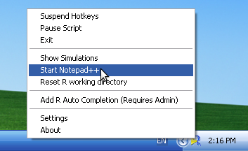
- Start Notepad++ (and R) by right clicking on the NppToR icon in the Windows Task Tray and selecting 'Start Notepad++'
RStudio
Features
- Syntax highlighting - text colored according to syntax rules
- Specifically designed for R
- Bracket matching
- Console integrated
- Cross platform
- Submit (Run) code line-by-line or selected lines (Cntr-ENTER)
- Submit (Run) all code (Cntr-Shift-ENTER)
- Auto-complete (Cntr-SPACE)
- Parameter prompting and integrated help (Cntr-SPACE)
- Live workspace
- Live command history
- Fully integrated File manager
- Intuitive and user-friendly package manager
- Integrated R help browser
Installation and setup
- Download Notepad ++ from here
- Select the installation package recommended for your system (e.g. 'RStudio Desktop 0.93.84 - Windows XP/Vista/7')
- Click 'Run' and when prompted verify the publisher
- Use all of the defaults while installing
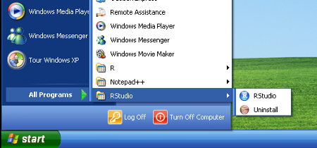
- Start RStudio from the Windows Start Menu
HowTo's
- Start a new script
- File->New->Rscript
Emacs
| Feature | Notepad ++ | RStudio | Emacs |
|---|---|---|---|
| Platform | Win only | Win,Mac,Linux | Win,Mac,Linux |
| Syntax Highlighting | Yes | Yes | Yes |
| Bracket matching | Yes | Yes | |
| Integrated Console | No | Yes | Yes |
| Auto-complete | Yes | Yes | Yes |
| Parameter prompting and integrated help | No | Yes | No |
| Code folding | Yes | No | Yes |