This section builds on the study of
shear bands as a function of the friction F
and dilation angles Y.
Here, the
distribution in mean
stress is investigated as a function of rock properties, layering and
the presence of fluids.
MODEL SET UP
The model is a horizontal plane at a fixed lithostatic pressure (
p),
fluid absent and is deformed in pure shear with a horizontal shortening
axis. The bulk modulus,
K,
and
shear
modulus G
are such that they yield a Poisson ratio
n
= 0.25 and
l
=
G.
Fluids in the pores
are included in some calculations at different pore pressures, and a
horizontal layer with different elastic moduli is added in some
calculations.
 Input
file
Input
file
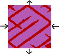
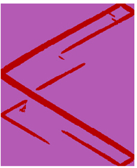
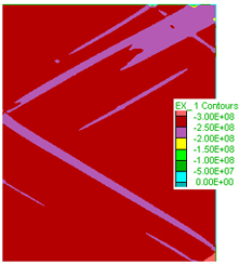
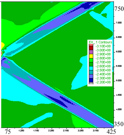
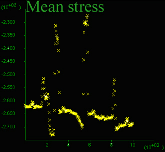
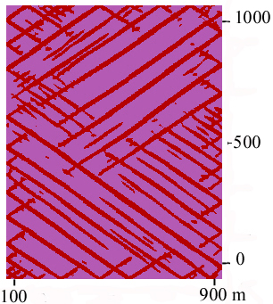
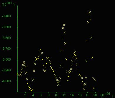
Figure 1. Study of pressure
drop in model 16 (equal model 15), step
55000. Drop in stress within the shear bands
is of the order of 0.3-0.5 kbar (Figures B, C and D).
A) State
|
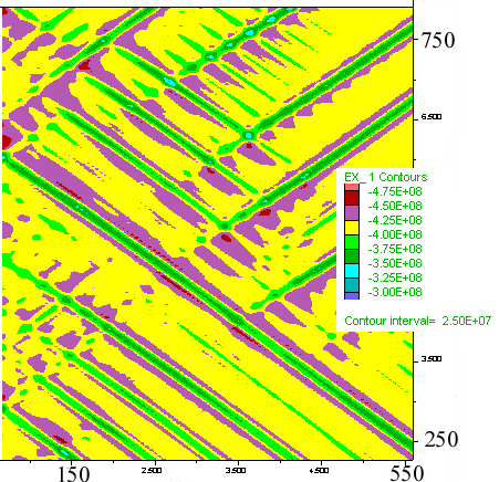
B) Mean stress
distribution
|
C) Mean stress zoom
|
D) Vertical profile of
mean stress
|
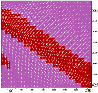
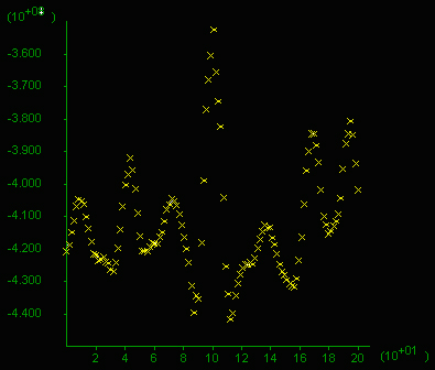
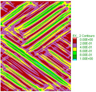
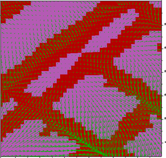
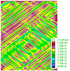
Figure 2. Model 19. Same as
Figure 1 in the presence of pore fluids
at hydrostatic pressure. Step 68000. A) State. Much
narrower and numerous shear bands develop compared to the case with no
fluids (Fig. 1). Click on figure for movie. B) Is a zoom of a shear
band
in A) and shows the fluid flow vectors indicating flow into the shear
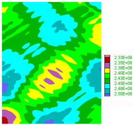
bands. C) Mean stress distribution in a typical area approximately a
quarter of the box area.
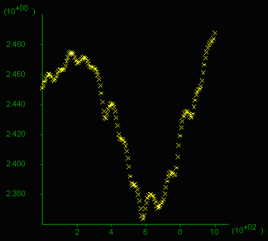
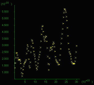
D) Mean stress in 10^8 Pa (=1 kbar) and the x-axis is in meters on the
vertical (only 200 m section plotted). Note the difference between
highs and lows reaches almost 1 kbar and values oscilate around 4 kbar
at this stage.
Click on figure to see a movie of the mean stress evolution.
F) Total volume flux vertical profile (in m3), x-axis in 100m. Shear
zones have seen an order magnitude
more fluid than its surroundings, this is a result of the dilation
angle of 20o
used.
In these models there is no increase in permeability due to yielding
and no fluid source.
A) State (movie)
|
B) Zoom of A) plus flow
vectors
|
C) Mean stess
|
D) Mean stress profile
(movie)
 |
E) Total volume flux
|
F) Vertical profile
volume flux
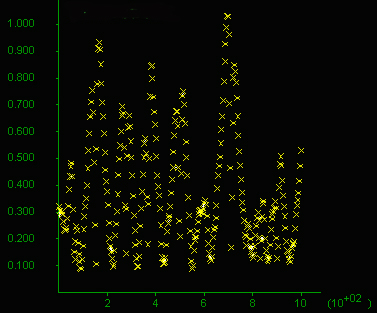 |
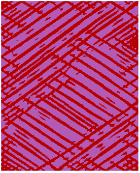
Figure 3. Model 20. Like
Figure 2 but pore fluids are initially at
twice hydrostatic pressure. Step 55000. A) State. Much
narrower and numerous shear bands develop compared to the case with no
fluids (Fig. 1). Click on figure for movies. B) Is a zoom of a shear
band
in A) and shows the fluid flow vectors indicating flow into the shear
bands. C) Pore pressure distribution showing a minimum in the center of
the box.
D) Pore pressure profile showing a variation of 0.12 kbar across the
area.
E) Mean stress distribution in a typical area approximately a quarter
of the box area.
F) Mean stress given in 10^8 Pa (=1 kbar) along a vertical section
(x-axis in m), 200 m long through the middle of the box. Note the
difference between highs and lows reaches 0.8 kbar and values oscilate
around 4 kbar at this stage.
Click on figure to see a movie of the mean stress evolution.
G) Total volume flux vertical profile (in m3), x-axis in 100m.
H) Volume flux profile.
A) State (movie)
|
B) Zoom of A) plus flow
vectors
|
C) Pore pressure (movie)
|
D) Pore pressure profile
(movie)
|
E) Mean stess 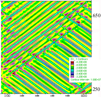
|
F) Mean stress profile
(movie)
|
G) Volume Flux
|
H) Volume Flux Profile
|