Appears in: Nineteenth International Conference on Machine Learning (ICML-2002), Sydney, Australia, 8-12 July 2002.
L. J. Fitzgibbon, D. L. Dowe and L. Allison
School of Computer Science and Software Engineering
Monash University, Clayton, 3168
Australia
The Minimum Message Length (MML) principle is an invariant Bayesian point estimation technique based on information theory. The basic tenet of MML is that the hypothesis (or model or distribution) which allows for the briefest encoding of the data in a two-part message is the best explanation of the data. This view of inference as a coding process leads to discretisation of the hypothesis space and a message length, which gives an objective means to compare hypotheses. The message length is a quantification of the trade-off between model complexity and goodness of fit that was first described by [10]. Since their seminal paper various approximations and derivations have appeared under the veil of Minimum Message Length (MML) [12,11] or Minimum Description Length (MDL) [6].
MML87 [12] has recently been applied to the problem of model selection in univariate polynomial regression with normally distributed noise by [8]. It was compared against Generalised Cross-Validation (GCV), Finite Prediction Error (FPE), Schwartz's Criterion (SCH), and VC Dimension and Structural Risk Minimisation (SRM) [7] over a set of polynomial and non-polynomial target functions, and for a range of noise levels. The criterion used to judge the performance of the different methods was Squared Prediction Error (SPE). In their results, the MML method had the smallest average SPE of all the methods for all target functions and noise levels. SRM was close behind. The other methods - GCV, FPE and SCH - had squared prediction error in the order of 100 times that of MML and SRM.
The Message from Monte Carlo (MMC) algorithm has been recently described in [1]. It uses the posterior as an importance sampling density to implicitly define uncertainty regions, for which message lengths can be approximated using Monte Carlo methods. Here, we apply MMC to univariate polynomial regression using discrete orthonormal polynomials and compare it with the two best contenders from [8]: MML87 and SRM.
The MMC algorithm, Dowe's MMLD approximation and Wallace's FSMML Boundary Rule are given in Section 2. The polynomial model and Bayesian priors are given in Section 3. A reversible jump Markov chain Monte Carlo algorithm for sampling polynomials is described in Section 4. Experimental evaluation is contained in Section 5 and the conclusion in Section 6.
In this section we describe the Message from Monte Carlo (MMC) algorithm. Many of the mathematical results for this algorithm are omitted due to space; see [1] for more information. The algorithm approximates the length of an optimal two-part message that would, in principle, allow for the transmission of some observed data over a noiseless coding channel. The first part of the message contains a code-word that represents a model and the second part of the message contains the data encoded using the stated model.
We use a Bayesian setting where the sender and receiver agree on a prior distribution ![]() and likelihood function
and likelihood function
![]() over the parameter space,
over the parameter space, ![]() , and data space,
, and data space, ![]() . We use the same notation for a vector of values as we do for a single value (i.e.
. We use the same notation for a vector of values as we do for a single value (i.e. ![]() and
and ![]() can be vector values). When we talk about regions, or uncertainty regions, of the parameter space, we mean arbitrary sets of elements from the parameter space (i.e.,
can be vector values). When we talk about regions, or uncertainty regions, of the parameter space, we mean arbitrary sets of elements from the parameter space (i.e.,
![]() ). The parameter space can be a union of subspaces of different dimension.
). The parameter space can be a union of subspaces of different dimension.
The MMC algorithm uses Dowe's MMLD message length approximation - described in [5] - to calculate message lengths. For some arbitrary set of models from the parameter space, ![]() , MMLD approximates the length of the first part of the message as the negative log integral of the prior over
, MMLD approximates the length of the first part of the message as the negative log integral of the prior over ![]() , and the length of the second part as the expected value (with respect to the prior), over
, and the length of the second part as the expected value (with respect to the prior), over ![]() , of the negative log-likelihood. This gives rise to an MMLD message length of
, of the negative log-likelihood. This gives rise to an MMLD message length of
The objective of the MMC algorithm is to find the region, ![]() , of the parameter space which minimises the MMLD message length expression. To do so, we need to be able to compute the necessary integrals in Equation 1 accurately and efficiently over a possibly high-dimensional space. The MMC solution is based on posterior sampling and Monte Carlo integration.
, of the parameter space which minimises the MMLD message length expression. To do so, we need to be able to compute the necessary integrals in Equation 1 accurately and efficiently over a possibly high-dimensional space. The MMC solution is based on posterior sampling and Monte Carlo integration.
The optimal region of the parameter space will consist of models with high posterior probability. We therefore draw a sample
![]() from the posterior distribution of the parameters
from the posterior distribution of the parameters ![]() using the appropriate sampler for some
using the appropriate sampler for some ![]() . The sample can contain models of variable dimension.
. The sample can contain models of variable dimension.
The uncertainty region, ![]() , can be implicitly defined by choosing a subset of the sample,
, can be implicitly defined by choosing a subset of the sample,
![]() , where we consider
, where we consider ![]() to be a subset of the true (explicit) region,
to be a subset of the true (explicit) region,
![]() .
. ![]() is a finite set and we can therefore approximate the terms in the MMLD message length equation (Equation 1) using Monte Carlo integration. These terms require a sample from the prior distribution of the parameters. For example, the expectation in the second part uses the prior, and the integral in the first part can be approximated by the proportion of the sample that falls within the uncertainty region,
is a finite set and we can therefore approximate the terms in the MMLD message length equation (Equation 1) using Monte Carlo integration. These terms require a sample from the prior distribution of the parameters. For example, the expectation in the second part uses the prior, and the integral in the first part can be approximated by the proportion of the sample that falls within the uncertainty region, ![]() . However, we are sampling from the posterior because we expect the optimal uncertainty region to consist of models with high posterior probability. We use the posterior as an importance sampling density [2] and we weight the sample so that it is distributed as if being generated from the prior.
. However, we are sampling from the posterior because we expect the optimal uncertainty region to consist of models with high posterior probability. We use the posterior as an importance sampling density [2] and we weight the sample so that it is distributed as if being generated from the prior.
Converting the MMLD message length expression into its equivalent (unnormalised) probability (by taking
![]() of Equation 1) we get
of Equation 1) we get
 |
(2) |
It can be seen that the region that minimises the MMLD message length is the region that maximises the product of the integral of the prior probability of models in the region and the weighted geometric mean of the likelihood (weighted by the prior). As the sample size increases, the uncertainty region will typically become smaller and converge to the posterior mode (MAP) estimate. So, while we wish to compute expectations over the uncertainty region weighted by the prior, we know that the uncertainty region will contain models with high posterior probability. For this reason, importance sampling will allow us to evaluate the sums in Equations 3 and 4, even for large amounts of observed data and where the likelihood function is very concentrated. Or, to put it another way, when the importance sampling density is very concentrated, it is concentrated in the area where we wish to do the Monte Carlo integration.
We expect (but do not require) that the prior will integrate to unity. Therefore, the length of the first part of the MMLD message can be approximated by the negative logarithm of the proportion of the weighted sample that falls within the region
The length of the second part of the MMLD message is the expected value of
![]() over the region,
over the region, ![]() , with respect to the prior
, with respect to the prior ![]() . This can be approximated using a Monte Carlo integration using the elements of the (weighted) sample that fall within the region,
. This can be approximated using a Monte Carlo integration using the elements of the (weighted) sample that fall within the region, ![]()
The total MMC message length is the sum of Equations 3 and 4.
Attempting to minimise the MMLD equation analytically (Equation 1) yields the following MMLD `Boundary Rule' (e.g., see [5])
where the boundary,
![]() , of
, of ![]() , is an iso-likelihood contour of
, is an iso-likelihood contour of ![]() . In other words, the values of
. In other words, the values of
![]() and of
and of
![]() are constant on
are constant on
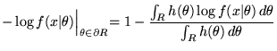
![]() . The MMLD Boundary Rule states that for the region which minimises the message length, the negative log-likelihood at the boundary of
. The MMLD Boundary Rule states that for the region which minimises the message length, the negative log-likelihood at the boundary of ![]() is equal to one plus the expected negative log-likelihood over the region weighted by the prior.
is equal to one plus the expected negative log-likelihood over the region weighted by the prior.
An iso-likelihood contour is defined by a single continuous parameter representing the log-likelihood of models on the boundary of the region,
![]() . The Monte Carlo integrations of the message length terms are a discrete function of the boundary. It is therefore sufficient to consider that one or more of the models in the sample,
. The Monte Carlo integrations of the message length terms are a discrete function of the boundary. It is therefore sufficient to consider that one or more of the models in the sample, ![]() , lie on the boundary.
, lie on the boundary.
The number of possible iso-likelihood contours in the sample is equal to the number of distinct values of the likelihood that appear in the sample. If we sort the sample into descending order of likelihood - starting at the maximum - then an iso-likelihood contour is given by a boundary index into the sample vector. For example, let ![]() denote a boundary index into the sample vector. This means that
denote a boundary index into the sample vector. This means that ![]() is on the iso-likelihood boundary,
is on the iso-likelihood boundary,
![]() , and the corresponding uncertainty region is
, and the corresponding uncertainty region is
since the sample has been ordered (i.e.
![]() ).
).
The MMLD Boundary Rule (Equation 5) states that the negative log-likelihood of models on the boundary of the region is equal to the prior-weighted average negative log-likelihood of models in the region plus one. Therefore, by Monte Carlo integration using the elements of the (importance weighted) sample that fall into ![]() , the rule becomes
, the rule becomes
 |
(6) |
In order to find the optimal boundary index, we start with the maximum likelihood model and continue to increase the boundary index while the boundary model's negative log-likelihood is less than one plus the average over the region. In other words, we start with
![]() , and end up with
, and end up with
![]() where
where
![]() is greater than the average negative log-likelihood over
is greater than the average negative log-likelihood over
![]() plus one.
plus one.
This will give us an implicit region that minimises the MMLD message length. However, use of this method will build regions that do not approximate efficient code-book entries because the region will be (wholly) determined by the likelihood of the observed data (which the receiver does not know) and will (generally) be unsuitable for encoding future data. In order to approximate a decodeable, efficient code-book we must ensure that the region consists of models with similar distributions. To do so, we use Wallace's FSMML Boundary Rule [9][Chapter 4]
 |
(7) |
where
![]() is the point estimate for the region, and
is the point estimate for the region, and
![]() is the Kullback-Leibler distance of
is the Kullback-Leibler distance of
![]() from
from ![]() . How can the FSMML Boundary Rule's dependence on the point estimate,
. How can the FSMML Boundary Rule's dependence on the point estimate, ![]() , be resolved and the rule used efficiently? The approach that we take is to begin with the maximum likelihood estimate, and as we add new members to the region, we allow them to compete for the right to become the point estimate of the region. If the new member is able to encode the data that can arise from the models in the region more efficiently, on average, than any other member of the region, then it wins the right to be the point estimate. The estimate therefore converges as the uncertainty region grows.
, be resolved and the rule used efficiently? The approach that we take is to begin with the maximum likelihood estimate, and as we add new members to the region, we allow them to compete for the right to become the point estimate of the region. If the new member is able to encode the data that can arise from the models in the region more efficiently, on average, than any other member of the region, then it wins the right to be the point estimate. The estimate therefore converges as the uncertainty region grows.
We can now describe the MMC algorithm in full. We draw a sample
![]() from the posterior distribution of the parameters
from the posterior distribution of the parameters ![]() using the appropriate sampler for some
using the appropriate sampler for some ![]() . The sample can contain models of variable dimension. First, the sample is ordered in descending order of likelihood. We now allocate space for a boolean array that indicates whether an element of the sample has been allocated to a region. Each element of the allocated array gets initialised to false. We begin the iteration by finding the unallocated model of maximum likelihood. Since the sample has been sorted, this is simply the first unallocated element of the sample. Denote this by
. The sample can contain models of variable dimension. First, the sample is ordered in descending order of likelihood. We now allocate space for a boolean array that indicates whether an element of the sample has been allocated to a region. Each element of the allocated array gets initialised to false. We begin the iteration by finding the unallocated model of maximum likelihood. Since the sample has been sorted, this is simply the first unallocated element of the sample. Denote this by ![]() . We begin to grow the first region by starting with
. We begin to grow the first region by starting with ![]() and then initialise the estimate for the region,
and then initialise the estimate for the region,
![]() , to
, to ![]() . We also initialise variables to calculate the necessary sums in the MMC message length equation (Equations 3 and 4). We continue to increment the pointer,
. We also initialise variables to calculate the necessary sums in the MMC message length equation (Equations 3 and 4). We continue to increment the pointer, ![]() , until we find the boundary
, until we find the boundary ![]() (i.e. until the MMLD Boundary Rule fails). For each value of
(i.e. until the MMLD Boundary Rule fails). For each value of ![]() we also check that the model
we also check that the model ![]() fulfils the FSMML Boundary Rule. If it does, then we flag it as being allocated to the region. We next consider it as a candidate for the point estimate. If the prior-weighted expected Kullback-Leibler distance between the models in the region and this candidate is less than the equivalent for the currently reigning estimate then the candidate becomes the point estimate.
fulfils the FSMML Boundary Rule. If it does, then we flag it as being allocated to the region. We next consider it as a candidate for the point estimate. If the prior-weighted expected Kullback-Leibler distance between the models in the region and this candidate is less than the equivalent for the currently reigning estimate then the candidate becomes the point estimate.
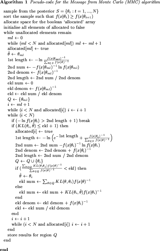
Each time we increment the pointer, we update the length of the first part of the message, the average over the region (Length of MMC 2nd Part) and the expected Kullback-Leibler distance in constant time. Once the MMLD Boundary Rule is violated, we reconsider all unallocated models to the left (i.e. ![]() ) since the estimate may have changed and some models that now deserve to be in the region may have previously been rejected on the first pass. After this second pass, we store all of the results and begin growing a new region using the first unallocated element of the sample (the model of maximum likelihood). This is repeated until all elements of the sample have been assigned to a region. Pseudo-code for the algorithm is given as Algorithm 1.
) since the estimate may have changed and some models that now deserve to be in the region may have previously been rejected on the first pass. After this second pass, we store all of the results and begin growing a new region using the first unallocated element of the sample (the model of maximum likelihood). This is repeated until all elements of the sample have been assigned to a region. Pseudo-code for the algorithm is given as Algorithm 1.
The MMC algorithm returns a set of regions with associated point estimates and message lengths. If the objective is to select a single model, then the point estimate from the region with the minimum message length is chosen. If the objective is to compute the average of some quantity of interest under the posterior, then Bayesian Model Averaging can be performed at reduced computational cost using the set of point estimates weighted using their message lengths.
The algorithm is computationally feasible because, when attempting to build the region associated with
![]() , the potential candidates for the region must pass the MMLD Boundary Rule. Therefore, the number of candidates presented to the FSMML Boundary Rule is considerably reduced.
, the potential candidates for the region must pass the MMLD Boundary Rule. Therefore, the number of candidates presented to the FSMML Boundary Rule is considerably reduced.
When a candidate model is accepted as a member of the region, we compute the expected Kullback-Leibler distance between the existing members of the region and the candidate. This would appear to be an expensive step. However, this sum need only be carried out while it (the partial sum) is less than the expected Kullback-Leibler distance to the current point estimate. The importance weighting gives the Kullback-Leibler distance between models with small likelihoods more weight, so the sum should be performed in ascending order of likelihood so that it (the partial sum) is likely to exceed the current EKL sooner. This strategy was found to yield an efficient algorithm in our experiments.
All that the MMC algorithm requires to operate is a sample from the posterior distribution and a function for computing the Kullback-Leibler distance. It can therefore be viewed as a posterior sampling post-processing algorithm. Markov Chain Monte Carlo (MCMC) [3] methods can be used to do the sampling.
We now describe the polynomial model and priors that we use in the experimental evaluation. The likelihood function for the ![]() observations
observations
![]() is
is
| (8) |
where  |
(9) |
The basis functions, ![]() 's, are orthogonal with respect to the data:
's, are orthogonal with respect to the data:
![]()
![]() and normalised to unity
and normalised to unity
![]() (i.e. generalised Fourier series).
(i.e. generalised Fourier series).
We use two different priors on the generalised Fourier series coefficients
![]() . Prior 1 is the same prior that [8] used - an (independent) Gaussian prior on each coefficient
. Prior 1 is the same prior that [8] used - an (independent) Gaussian prior on each coefficient
where  |
(11) |
The prior reflects the belief that we expect each of the coefficients and noise to (roughly) contribute to the observed variance of the ![]() values equally. We note that [8] use the same prior, and that the difference between their
values equally. We note that [8] use the same prior, and that the difference between their ![]() and our
and our ![]() arises because they normalise the average inner-product of their basis functions.
arises because they normalise the average inner-product of their basis functions.
The second prior that we use on the coefficients is a uniform additive prior
where  |
(13) |
This reflects the belief that a coefficient could `explain' the variance that lower order coefficients have not, and that there is no preference for a specific value over the range
![]() .
.
We use a diffuse inverted gamma prior on ![]() (for conjugacy):
(for conjugacy):
![]() , and a geometric prior on the order of the model:
, and a geometric prior on the order of the model:
![]() .
.
To sample from the posterior we use Green's reversible jump MCMC methodology [4].
Let ![]() denote the upper bound on the order of the polynomials under consideration. The sampler consists of three types of moves: birth to a higher dimension, death to a lower dimension and move in the current dimension. We find that the sampler mixes better when allowed to jump more than one order when a birth or death dimension change move is made. So when a birth move is performed on a k-order model, the new order is generated from a
denote the upper bound on the order of the polynomials under consideration. The sampler consists of three types of moves: birth to a higher dimension, death to a lower dimension and move in the current dimension. We find that the sampler mixes better when allowed to jump more than one order when a birth or death dimension change move is made. So when a birth move is performed on a k-order model, the new order is generated from a
![]() distribution which has been normalised over
distribution which has been normalised over
![]() . This is mirrored for the death step over the interval
. This is mirrored for the death step over the interval
![]() .
.
For each sweep of the sampler we randomly choose between the ![]() move types:
move types:
![]() , where
, where ![]() denotes the move step (no dimension change), and
denotes the move step (no dimension change), and ![]() denotes a jump to an m'th order polynomial. We denote the probability of each move conditional on
denotes a jump to an m'th order polynomial. We denote the probability of each move conditional on ![]() (the order of the last polynomial in the chain) as
(the order of the last polynomial in the chain) as ![]() . The probabilities of birth, death and move are denoted by
. The probabilities of birth, death and move are denoted by ![]() ,
, ![]() , and
, and
![]() respectively and are independent of
respectively and are independent of ![]() and chosen by the practitioner1. Therefore
and chosen by the practitioner1. Therefore ![]() satisfies2 the following:
satisfies2 the following:
![]() ,
,
![]() , and
, and
![]() for
for ![]() . We now detail the samplers for each of the three move types.
. We now detail the samplers for each of the three move types.
For the move step the new values for the coefficients and ![]() are generated by Gibbs sampling. In describing the full conditional for coefficients we use the notation
are generated by Gibbs sampling. In describing the full conditional for coefficients we use the notation ![]() to represent the set of all coefficients except
to represent the set of all coefficients except ![]() (i.e.
(i.e.
![]() and
and ![]() ).
).
The full conditional distribution for coefficient ![]() using Prior 1 (Equation 10) is
using Prior 1 (Equation 10) is
 |
(14) |
![]() is normally distributed with mean
is normally distributed with mean
![]() and standard deviation
and standard deviation
![]() .
.
The full conditional distribution for coefficient ![]() over the range
over the range
![]() using Prior 2 (Equation 12) is
using Prior 2 (Equation 12) is
| (15) |
![]() is normally distributed with mean
is normally distributed with mean
![]() and standard deviation
and standard deviation
![]() .
.
The full conditional distribution for ![]() is
is
| (16) |
which is an inverted gamma distribution with parameters:
![]() and
and
![]() .
.
The birth and death steps require dimension matching. If we jump from a ![]() 'th order polynomial to an
'th order polynomial to an ![]() 'th order polynomial then the new coefficients are sampled using Gibbs sampling. To create the necessary bijection between the two spaces we generate
'th order polynomial then the new coefficients are sampled using Gibbs sampling. To create the necessary bijection between the two spaces we generate ![]() variables from an
variables from an ![]() distribution.
distribution.
| (17) |
Using Green's notation the acceptance probability of the move is
| (18) |
The proposal ratio is the same for both Prior 1 and 2
proposal ratio |
(19) |
The Jacobian for Prior 1 is
 |
(20) |
and the Jacobian for Prior 2 is
 |
(21) |
The acceptance probability for the death step is the inverse of the acceptance probability for the birth step.
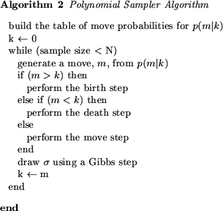
The sampler begins with a zero order least squares model. The algorithm (![]() is the order of the last polynomial in the chain) is given in Algorithm 2.
is the order of the last polynomial in the chain) is given in Algorithm 2.
The MMC algorithm needs to be able to compute the Kullback-Leibler (KL) distance between two models to build the regions. Since each ![]() is independent, the KL distance for a polynomial model is the sum of Gaussian KL distances taken at each known
is independent, the KL distance for a polynomial model is the sum of Gaussian KL distances taken at each known ![]() . Given the true model
. Given the true model
![]() and inferred model
and inferred model
![]() , the (analytical) KL distance simplifies to
, the (analytical) KL distance simplifies to
 |
(22) |
where
![]()
![]() and
and
![]()
![]() . The KL distance for generalised Fourier series can be computed in
. The KL distance for generalised Fourier series can be computed in
![]() time.
time.
Some example analyses using the MMC algorithm are shown in Figures 1 to 3. The graphs show the generated data3 as crosses and the fitted function with the estimated noise represented at plus and minus one standard deviation. For this simple example we increased the number of data points, ![]() , from 10 to 20 to 40. We see that MMC is able to choose a model whose complexity is suitable for the given data.
, from 10 to 20 to 40. We see that MMC is able to choose a model whose complexity is suitable for the given data.
We compare the MMC method with two other inference methods on a set of polynomial and non-polynomial target functions. We use the same target functions as [8] and also include some low order polynomials. The target functions are illustrated in Figure 4. Each method is given noisy data generated from the known target function, and is required to infer a single polynomial up to order 20. We use the Squared Prediction Error (SPE) criterion to measure the performance of the methods.
The following methods are included in the evaluation: MMC using Prior 1 (MMC-1); MMC using Prior 2 (MMC-2); Minimum Message Length (MML87) [8]; and Structural Risk Minimization (SRM) [7]. For the MMC methods we sample 3000 polynomials from the posterior, the first 500 being discarded as burn-in.
The experiment consisted of 1000 trials for ![]() and
and ![]() , and for high and low noise values. High noise is defined as a Signal to Noise Ratio (SNR) of 0.78125 where the SNR is defined as the second moment of the function about zero divided by the noise. Low noise is defined as an SNR of 100. Due to the number of results, they could not all be included (see [1] for more). A subset of the results are displayed in a boxplot (Figure 5). The boxplot is of the natural logarithm of the SPE, because the log-SPE data looked to be normally distributed upon inspection. Each box shows the lower quartile, median and upper quartile.
, and for high and low noise values. High noise is defined as a Signal to Noise Ratio (SNR) of 0.78125 where the SNR is defined as the second moment of the function about zero divided by the noise. Low noise is defined as an SNR of 100. Due to the number of results, they could not all be included (see [1] for more). A subset of the results are displayed in a boxplot (Figure 5). The boxplot is of the natural logarithm of the SPE, because the log-SPE data looked to be normally distributed upon inspection. Each box shows the lower quartile, median and upper quartile.
The subset of results presented was chosen because it is representative of the majority of the omitted results. The MMC method was found to have lower SPE medians, and better inter-quartile ranges, on average, than MML87 and SRM. The MMC results where almost identical for the two priors used. We note that our results may be interpreted differently to those presented in [8] because they plot the average SPE, for which MML87 outperforms SRM.
We have applied the Message from Monte Carlo (MMC) inference method (using the MMLD approximation and FSMML Boundary Rules) to univariate polynomial model selection. The MMC method was compared with Structural Risk Minimisation (SRM) and Minimum Message Length (MML87) and was found to have the lowest median Squared Prediction Error (SPE) (on average) for data generated from a range of polynomial and non-polynomial target functions. The MMC algorithm is flexible, only requiring a sample from the posterior distribution and a means of calculating the Kullback-Leibler distance. This generality allows it to be easily applied to new and difficult problems.
This document was generated using the LaTeX2HTML translator Version 2K.1beta (1.57)
Copyright © 1993, 1994, 1995, 1996,
Nikos Drakos,
Computer Based Learning Unit, University of Leeds.
Copyright © 1997, 1998, 1999,
Ross Moore,
Mathematics Department, Macquarie University, Sydney.
The command line arguments were:
latex2html -local_icons -notransparent -white -antialias -nonavigation -split 0 icml.tex
The translation was initiated by Leigh Fitzgibbon on 2002-05-27
![\begin{figure}\centering\includegraphics[width=240pt]{/home/leighf/static/Paper-ICML2002/example_quintic_10_1}
\end{figure}](img124.png)
![\begin{figure}\centering\includegraphics[width=240pt]{/home/leighf/static/Paper-ICML2002/example_quintic_20_1}
\end{figure}](img125.png)
![\begin{figure}\centering\includegraphics[width=240pt]{/home/leighf/static/Paper-ICML2002/example_quintic_40_1}
\end{figure}](img126.png)
![\begin{figure}\centering\includegraphics[width=240pt]{/home/leighf/static/Paper-ICML2002/targetfns}
\end{figure}](img128.png)
![\begin{figure}\centering\includegraphics[width=240pt]{/home/leighf/static/Paper-ICML2002/res_noise_10_p3_spe}
\end{figure}](img130.png)