^CSE454^ ^Local^ ^Sample-Q's^ & ^MML^

CSE454 Data Mining and MML 2004

Computer Science and Software Engineering, Monash University, Australia,
CSE454 Data Mining and MML (semester 1), 17th June 2004

Note: The tables are always given out, for a reason -- become familiar with them. Show working, and perhaps give a little explanation, so that credit can be given even if a small slip makes an estimate wrong. But also do a quick "sanity check" to make sure that a numerical answer is plausible.

1. Briefly define the following terms as used in the module CSE454 `Data Mining and MML':
  1. Prior probability.
  2. Nit (also known as nat).
  3. Likelihood.
  4. Posterior odds-ratio (of H1 and H2, say).
  5. Entropy
[(total) 10 marks]
Notes on answers.

Not an answer, a note: Entropy can be interpreted as the expected (average) information content per item of a sample drawn from a probability distribution. In later questions, e.g. Q2, do not confuse entropy with the total information content of a given data-set (i.e. many data).


2. (a) There are three "obvious", efficient ways to encode a univariate data-set over a finite alphabet: An "adaptive" code, and two other methods. What are the two other methods?
[(a): 2 marks]
(b) How do the message lengths under the three methods compare?
[(b) 3 marks]
(c) An experiment has one of three results {A,B,C}. The experiment is repeated several times giving this set of results:
A, B, A, C, B, A, C, B, A, A
Show how the adaptive method would operate for this set, and thus estimate the information content of the data-set.
[(c) 10 marks]
[(total) 15 marks]
Notes on answers.

The alphabet is of size three (remember this for Q3).

(c) Adaptive method, 10 data, 5×A, 3×B, 2×C:

       A   B   A   C   B   A   C   B   A   A
 #A: 1   2   2   3   3   3   4   4   4   5   6   -- green
 #B: 1   1   2   2   2   3   3   3   4   4   4   -- black
 #C: 1   1   1   1   2   2   2   3   3   3   3   -- blue
Tot: 3   4   5   6   7   8   9  10  11  12  13

       1   1   2   1   2   3   2   3   4   5     5! 3! 2!
       -   -   -   -   -   -   -  --  --  --  =  --------
       3   4   5   6   7   8   9  10  11  12     12! / 2

  ln(12!) - ln(5!) - ln(3!) - ln(2!) - ln(2)
= 20.0    - 4.8    - 1.8    - 0.7    - 0.7
= 20.0 - 8.0
= 12.0 nits

(Sanity check to get an order of magnitude: If pr(A)=pr(B)=pr(C)=1/3 (and we don't actually know that!),   ln(3)~1.1; 1.1×10~11nits;  or  log2(3)=1.58; 1.58×10~16bits~11nits. Less something because the data is actually skewed, but plus something extra for the estimate of <pr(A),pr(B)>. Anything much bigger or much smaller is probably wrong.)


3. A certain bivariate data-set contains these two attributes: Attribute G can take the values {M,P,T}, and attribute D can take the values {R,U,S}. The frequencies of the various combinations are given in the table:
  D  
R U S G totals:
G M 6 2 2 10
P 3 4 3 10
T 1 3 6 10
  D totals: 10   9 11 (all: 30)
E.g. <M,R> occurs 6 times.
There is a suspicion that attribute D might depend on attribute G, although chance might have created that illusion. 
(a) How could the data be sensibly encoded under the hypothesis that there is no dependency? Estimate the information content of the data under that hypothesis. Show working.
[(a) 11 marks]
(b) How could the data be sensibly encoded under the hypothesis that attribute D is dependent on attribute G? Estimate the information content of the data under that hypothesis. Show working.
[(b) 11 marks]
(c) What do you conclude from (a) and (b) about the suspicion? Why?
[(c) 3 marks]
[(total) 25 marks]
Notes on answers.

In general, Bayes, dependent, P(G&D)=P(G).P(D|G)=P(D).P(G|D). If G and D are independent, P(G|D)=P(G), P(D|G)=P(D), so P(G&D)=P(G).P(D).

(a) One 3-state distribution for G and another 3-state distribution for D. All that practice in Q2 should remind you how to deal with multi-(3)-state distributions. Just follow the same process, twice. We want to see working and numbers.

(b) There are two possible ways to do part(b).
The first way is to use a 3-state distribution for G and three 3-state distributions for D: one when G=M, a second when G=P and a third when G=T. This makes 2 parameters for G and 3×2=6 parameters for D, total 8.
The second way is to code G×D as a 9-state distribution, giving 8 parameters for G and D together.
The first way seems slightly nicer and more in keeping with Bayes's theorem (Pr(D|G=M) etc.), and then the distribution for G is the same in part(a) & in part(b) which is handy for part(c) (i.e. it cancels out there)and you do only have 3-state distributions (see Q2) to deal with, but we wouldn't quibble under exam conditions. (The two ways of doing part(b), of which either one is sufficient, will not necessarily give exactly the same message length but they should be very close to each other.)

(c) The difference in the numbers from part(a) and part(b)....

(Sanity check: log2(3)=1.58 (ln(3)=1.1). There are sixty values over {M,P,T} or {R,U,S} to transmit in total. You should expect message length total of the same order of magnitude as 90bits (65nits) or thereabouts, maybe less, maybe more. But anything much bigger or much smaller is probably wrong.)


4. A data-set has the following attributes:
@0, Gender = Male | Female
@1, Married = W | S
@2, Party = Lib | Lab | Dem | Green | Indep
@3, SEG = L | M | H
@4, Z = P | N   -- predict
You want to infer a classification tree to predict @4 Z from @0 to @3.
(a) Briefly describe a general and efficient scheme for encoding classification trees over discrete and/or continuous input attributes, and discrete outputs.
[(a) 6 marks]
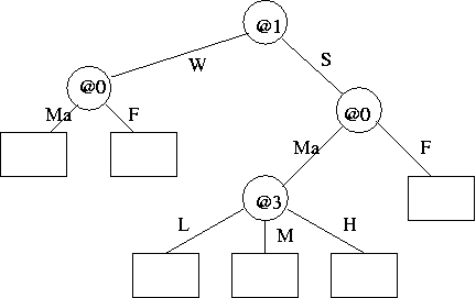
(b) Show how the structure of the following tree would be encoded (without data), and estimate its message length. Show working.
tree1
[(b) 6 marks]
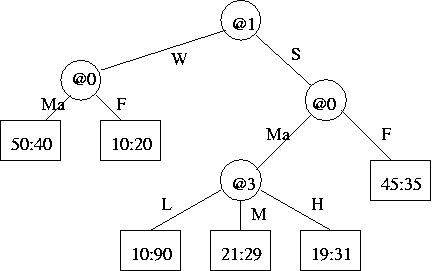
(c) The flow of data through the tree is shown below. Estimate the message length of the data (i.e. @4, Z) in the left-most leaf. Show working.
tree2
[(c) 6 marks]
(d) You are only now told that @3, SEG, is an ordered discrete type, i.e. L < M < H, it shares this (<) property of continuous attributes. This means that instead of 3-way splits, 2-way splits could be used on @3 SEG, i.e. {L} v. {M,H}, and {L,M} v. {H}. How would the tree encoding scheme be changed to deal efficiently with this new kind of attribute and split?
[(d) 8 marks]
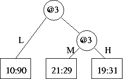
(e) Draw a new subtree that uses these new 2-way splits and is otherwise equivalent to (has the same leaves as) the subtree rooted at the old 3-way split in (c). What would the change in the total message length of tree and data be compared to the original scheme as used in part(a) to part(c)? Show working.
[(e) 7 marks]
(f) You will notice that in the new subtree you drew for part(e) the distributions of Z are very similar when SEG=M or when SEG=H. Estimate the change in the total message length if those two leaves of the new subtree are collapsed into one. Show working.
[(f) 7 marks]
[(total) 40 marks]

© 6/2003, L. Allison, School of Computer Science and Software Engineering, Monash University, Australia 3800. Created with "vi (Linux & IRIX)", charset=iso-8859-1
Notes on answers.

(a) Topology [how?], tests [how?]. Arity re tests on discrete attributes [how?]. Parameters of leaf distributions. Data (predicted) attribute(s) according to selected leaf model.
Don't forget, if a test-node tests a continuous attribute, that attribute can still be re-tested in subtrees of the test-node. (And looking ahead, you will have to quantify either the leaf parameter cost or, easier, the adaptive code (see Q2) under part(c).)

(b) Note that SEG's arity (three), doubtless as described for discrete tests in the answer to part(a), comes into play for the children of the test-node for @3. See the [tables] for log2 and/or ln of 2 and 3.

(c) Like Q2, except it is a simpler 2-state {P|N} distribution here, #P=50, #N=40. See the [tables] for Stirling's approximation to ln(n!) for n = 50, 40 and 91.

(d) This makes SEG "like" a continuous attribute in some ways. If tested, it is also necessary to code (1-bit for 3-state SEG) what the test condition is, i.e.  test1 = @3<M  or  test2 = @3<H. The new tests' arities are two, of course. And if tested, SEG can remain "active" in one of its subtrees, for one more test, but we wouldn't worry about that much in an exam.

(e) Here is the "the subtree rooted at the old 3-way split"
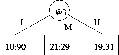
subtree

There are two possible trees that "use[s] these new 2-way splits" and are "otherwise equivalent to (have[s] the same leaves as)" it. Either one of the following would do:
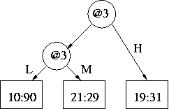
subtree
or subtree

(f) And here is the subtree if "those two leaves [when SEG=M, SEG=H] of the new subtree are collapsed into one."
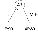
subtree

Under topology, we save one new-style split node on @3 and one leaf. The data part must change slightly corresponding to the move from 21:29 & 19:31 to 40:60; use those [tables] again. (Note that the SEG=L leaf and the rest of the tree, and their contributions to the message length, remain unchanged.)

(Sanity check: 100 data in the ratio 40:60 must cost very roughly 100-bits, 69-nits, i.e. numbers much bigger or much smaller must be wrong.)