1 Results from prior NSF support
Key
Connections in Arctic Aquatic Landscapes (NSF OPP-9615949, 1996-1999,
$1,962,905, PIs are J. Hobbie, A. Giblin, L. Deegan, and B. Peterson at the
Ecosystems Center, Woods Hole):
The goal of this study is to understand the
important connections that occur among different parts of the arctic aquatic ecosystem
including those from uplands to the riparian zone, from the riparian zone to
the surface waters, from the streams to lakes, and from the lakes to their
outlets. As a subcontractor on this
project Stieglitz ($75,000) is responsible for: (1) producing a computationally
efficient, physically based hydrology model that is effective in arctic
environments and is capable of simulating the flow of water from the hillslope
to the river network; (2) incorporating biological processes into the model
framework so as to predict the fluxes of CO2 and CH4
between the terrestrial landscape and the atmosphere, and the transport of
dissolved organic carbon (DOC) and nutrients to the rivers; and (3) scaling the
model results to large basins. Research
has focused on simulating the hydrology, growth and ablation of the snowpack,
and the evolution of the soil active layer at the Imnavait Creek watershed (2.2
km2), located in the Upper Kuparuk Basin of northern Alaska. To date one paper has been accepted to
Journal of Gepophysical Reviews [Stieglitz et al., 1999b] one paper is in revision at Global Biogeochemical
Cycles [Stieglitz et al., in review], one paper is in preparation [Stieglitz et al., in
preparation], and three presentationshave been given at AGU [Stieglitz
and Giblin, 1997; Stieglitz et al.,
1998; Stieglitz et al., 1999a] on topics ranging from simple hydrologic validations
at the watershed scale, to exploration of the feedbacks between soil moisture
evolution and the microbial decomposition of soil organic matter, to climate
change experiments.
Validation of Land Surface Hydrology
Parameterizations for Climate Models (NSF 9318896, EF Wood, PI):
This
work is relevant to the proposed research in that the goals of the former award
was to determine the relative performance of land surface hydrology
representations (models) appropriate for macroscale hydrologic modeling. The performance was assessed in terms of
their ability, to characterize 1) energy fluxes at the land surface, including
latent and sensible heat, outgoing short- and long-wave radiation, and ground
heat, and 2) the surface water budget, including soil moisture, infiltration,
and runoff production. The comparisons
were carried out within the context of the Project for Intercomparison of
Landsurface Parameterization Schemes (PILPS).
PILPS is sponsored by the WMO Committee on Atmospheric Sciences Working
Group on Numerical Experimentation and the Science Panel of the GEWEX
Continental- scale International Project.
The
first phase of the project was to evaluate the VIC-2L land-surface hydrological
model within the PILPS experiments.
This evaluation and intercomparison within PILPS allowed for systematic
testing of the model [Chen et al., 1997; Liang et al., 1996a; Pitman
et al., 1999] and indicated areas for improved parameterizations of
specific hydrological processes [Liang et al., 1996b; Liang et al., 1998; Peters-Lidard et al., 1998].
During the second phase of the project, a PILPS intercomparison experiment was conducted [Wood et al., 1998] based on 10 years of hourly data for 61 1x1 degree simulation grids representing the Red-Arkansas River basins in the southern great plains region of the United States. This experiment was the first PILPS intercomparison experiment using multiple years of observed meteorological data. Sixteen land surface hydrological models participated and detailed intercomparisons were carried out to evaluate the ability of the models to predict land-surface fluxes of water and energy at the scale of global atmospheric models [Liang et al., 1998; Lohmann et al., 1998a; Wood et al., 1998].
2 Relevant Arctic Programs
2.1 ARCSS, LAII, Flux Study
The
goal of the U.S. Arctic System Science
(ARCSS) Program is two-fold: (1) to understand the physical, biological,
and social processes of the arctic system that interact with the total Earth
system and thus contribute to or are influenced by global change, in order to
(2) advance the scientific basis for predicting environmental change on a
decades-to-centuries time scale and for formulating policy options in response
to the anticipated impact of changing climate on humans and social
systems. One of the three components of
the ARCSS was Land/Atmosphere/Ice/Interactions or LAII. Within LAII, four research areas were chosen
for initial emphasis: (1) arctic
feedback processes that may amplify global climate change; (2) changes in
arctic hydrological and biogeochemical systems; (3) changes in biotic communities;
and (4) regional and global effects of all these changes (the ARCC and LAII
goals are summarized from [ARCUS, 1993].
The
LAII Flux Study addressed some of these research areas. Its primary components were: (1) measurements
of fluxes of trace gases, water and energy between the arctic terrestrial
ecosystem and the atmosphere, and of the transport of water and materials to
the ocean, (2) determination of the primary controls on the fluxes, and (3)
scaling and synthesis to the regional scale [LAII-SMO, 1994]. Twelve individual projects made up the flux study
and were focused on the Kuparuk River basin as the study site. The long-term goals were to make predictions
of fluxes for the entire Arctic, based upon measurement techniques and models
developed. The goals of "Key Connections in Arctic Aquatic
Landscapes" are entirely
complimentary with the Flux Study.
2.2 Scaling up from small watersheds: ATLAS
A
recently funded LAII program is “Arctic Transitions in the Land-Atmosphere
System” (ATLAS). The overall goal of
this program is “to determine the geographical patterns and controls over
climate-land surface exchange (mass and energy) and to develop reasonable
scenarios for future climate change.”(ATLAS web site) Currently over a dozen projects are being funded, encompassing
both field research and modeling studies. The initial focus will concentrate on
the North Slope Western Transect that includes Barrow, Atquasuk, Oumalik, and
Ivotuk. Data collected by the various
groups will include water, energy, and trace gas fluxes between the terrestrial
landscape and the atmosphere, hydro-meteorological measurements, ground
temperatures and soil moisture status, soil respiration, etc. The modeling studies, which will make use of
data collected in the field projects, include permafrost models, the ARCSyM
regional climate model [Lynch et al., 1995], and a suite of ecosystem models such as GEM [Rastetter
et al., 1991], TEM [Raich et al., 1991], CENTURY [Parton et al., 1987], and SPA [Williams et al., 1996]. However, a major gap in this program that is
specifically identified is hydrology.
As stated in the ATLAS implementation document [ATLAS, 1998], “Many of the relevant parameters are to be measured
at the major tower sites. However,
there is currently no basis for estimating these parameters in a spatially
distributed fashion or in projecting these parameters into the future based on
reasonable scenarios of climatic change.
We need a project in meteorology and hydrology that focuses on spatial
and temporal patterns of climate and soil moisture, and considers the
relationship between these parameters and energy exchange and
runoff". The planning document
goes on to “… recommend that another project be added to focus on scaling of
hydrology to the regional scale. This
would make use of all the meteorology and soil moisture information from the
field research but would aggregate this information to produce sub-grid scale
fluxes and lateral transport at scales necessary for climate prediction.” A field study specifically aimed at
determining the spatial distribution of soil moisture is currently funded
(Hinzman, Goering, Kane).
We
propose here to fill this modeling gap in hydrology by making use of this
hydro-meterological data being collected in the field. We will use, as our starting point the
catchment based LSM that is currently being developed by the NASA NSIPP group.
Ultimately, this will lead to an improved seasonal and inter-annual variability
in climate simulations through a better representation of sub-grid scale
land-atmosphere water and energy fluxes.
The approach is computationally efficient, physically based, and can be
scaled to large watersheds. As a member
of the NASA collaboration Stieglitz will translate this modeling approach to
arctic regions using lessons learned from
the Arctic project "Key Connections in Arctic Aquatic Landscapes"
in the modeling of freeze-thaw processes, snow physics, and arctic hydrologic
processes.
3 Background
The
arctic climate system responds to external forcing from low latitudes but is
also driven by its own set of complex internal modes and feedbacks. Because these internal feedbacks are highly
non-linear, the Arctic is thought to be very sensitive to climate change. For example, with its high albedo and large
areal extent, snow cover on land can have considerable influence on regional
and hemispheric conditions. Furthermore, since the snowpack is
thermally insulating, and limits the otherwise efficient heat exchange between
the ground and the atmosphere, it controls the evolution of seasonal ground
temperatures. In turn, this thermal
control over the evolution of the hydrologically active soil depths plays a
large role in determining the magnitude and timing of spring melt water
delivered to the Arctic Ocean, which impacts stability to the surface layer,
and affects ocean circulation and seasonal sea ice formation. Finally, until the soil active layer deepen
into mineral soils, much of the water soil flows through a narrow zone in contact
with plant roots and soil organic matter, this having a direct influence on CO2
and CH4 fluxes, both greenhouse gasses. Hence, any long term forecast in a fully coupled climate system
is dependent on an accurate simulation of the land snow-covered area, snow
water equivalent, and permafrost dynamics.
Despite
the acknowledged role that the arctic system plays in regulating the planetary
climate, most land surface models intended for use in exploring the above
mentioned feedbacks (i.e., coupled with atmospheric circulation models, ocean,
and sea ice models) are inadequate.
Originally designed for mid-latitudes, most do not adequately represent
either snow physics or permafrost dynamics. Furthermore, no model to date
includes the role that topography plays in the development of soil moisture
heterogeneity and the critical, perhaps overwhelming, impact of this
heterogeneity on surface energy, water, and trace gas fluxes. Our objective is to correct these
deficiencies.
Given
the constraint that we wish to work with a Land Surface Model (LSM) that is
computationally efficient, can operate at large spatial and at high latitudes,
and eventually, be fully coupled within a GCM, the are number of models
available [Abramopoulos et al., 1988; Dickinson
et al., 1993; Koster and Milly,
1997; Koster and Suarez, 1996; Koster and Suarez, 1992a; Pitman and Desborough, 1996; Verseghy, 1996]. However, if
we do not wish to ignore the role topography plays in the development of soil
moisture heterogeneity and the impacts that this heterogeneity has on surface
water and energy fluxes, our options are limited. We can either account for the
topographic control over surface hydrology by explicitly modeling the movement
of water from the hillslopes to the valleys, which is computationally expensive
at even small spatial scales, or the impacts of topography can be modeled with
quasi-statistical techniques, such as those offered by TOPMODEL [Beven
and Kirkby, 1979; Sivapalan et al.,
1987] or VIC [Liang et al., 1994] formulations.
Both TOPMODEL and VIC formulations have now been used in conjunction
with sophisticated LSMs to successfully simulate the growth/ablation of the
seasonal snowpack, permafrost dynamics, and snowmelt and storm discharge at
scales ranging from small catchments to major river basins covering both the
arctic and boreal ecosystems. Modeling
results have been obtained for small arctic catchments [Stieglitz et al.,
1999b], large arctic basins including the Mackenzie [Bowling
and Lettenmaier, in press; Pauwels et
al., 1996], and the BOREAS boreal area ranging from tower scales
[Nijssen
et al., 1997; Pauwels and Wood,
1999a; Pauwels and Wood, 1999b] to regional scales [Pauwels, 1999]. Further, this type of modeling approach provides a
significant conceptual improvement over current, GCM soil column models, as
demonstrated by comparing site and simulated discharge [Betts and Viterbo,
2000; Pauwels, 1999; Stieglitz et al., 1997].
 The proposed work described
here will begin with the land surface model currently under development by the
NASA NSIPP program. This
catchment-based LSM was developed to overcome a critical deficiency in standard
General Circulation Model (GCM) based LSMs, namely, the neglect of an explicit
treatment for spatial variability in soil moisture. From the outset this work has been a collaborative effort between
NASA’s Goddard Institute for Space Studies (GISS), Lamont Doherty Earth
Observatory (LDEO: Marc Stieglitz, Colin Stark) and Goddard Space Flight Center
(GSFC: Randy Koster, Max Suarez, Agnes Ducharne, and Praveen Kumar). Using this model presents numerous
advantages to both NASA and NSF-OPP: (1) Leveraging off existing work avoids
expensive duplication of effort. (2) Because the approach uses the statistics
of the topography (via TOPMODEL formulations) rather than the details of the
topography, it is computationally efficient and numerically tractable at the
large spatial scales of today’s regional and global climate models. (3) The
limited validation performed to date indicates that the NASA LSM will be effective
in regions with permafrost [Stieglitz et al., 1999b] and significant snow cover (see Figure 3, [Stieglitz
et al., in preparation]. (4) In depth
validation in arctic regions-will provide NASA with invaluable insights into
the behavior of the model in a region that otherwise would receive only a
cursory validation.
The proposed work described
here will begin with the land surface model currently under development by the
NASA NSIPP program. This
catchment-based LSM was developed to overcome a critical deficiency in standard
General Circulation Model (GCM) based LSMs, namely, the neglect of an explicit
treatment for spatial variability in soil moisture. From the outset this work has been a collaborative effort between
NASA’s Goddard Institute for Space Studies (GISS), Lamont Doherty Earth
Observatory (LDEO: Marc Stieglitz, Colin Stark) and Goddard Space Flight Center
(GSFC: Randy Koster, Max Suarez, Agnes Ducharne, and Praveen Kumar). Using this model presents numerous
advantages to both NASA and NSF-OPP: (1) Leveraging off existing work avoids
expensive duplication of effort. (2) Because the approach uses the statistics
of the topography (via TOPMODEL formulations) rather than the details of the
topography, it is computationally efficient and numerically tractable at the
large spatial scales of today’s regional and global climate models. (3) The
limited validation performed to date indicates that the NASA LSM will be effective
in regions with permafrost [Stieglitz et al., 1999b] and significant snow cover (see Figure 3, [Stieglitz
et al., in preparation]. (4) In depth
validation in arctic regions-will provide NASA with invaluable insights into
the behavior of the model in a region that otherwise would receive only a
cursory validation.
4 Goals and Objectives
Research
programs focused on understanding the physical climate of high latitude
regions, and on predicting environmental change for these regions require a
sound basis for predicting the terrestrial water and energy budgets across a
range of spatial and temporal scales.
Unresolved is a clear understanding of the small scale processes and
features (e.g. topography, vegetation, soils) that must be included in such
terrestrial hydrologic models, including the importance of these small-scale
features for different seasons and the resulting errors if omitted. Thus, the
research will develop an integrated program that combines field measurements,
remote sensing observations and a terrestrial water-energy balance model with
the objectives:
(i) To
further our understanding of the relationship between the arctic ecosystem and
the physical climate system, with particular attention on understanding spatial
and temporal variability in water and energy fluxes.
(ii) To
study approaches for scaling processes to arctic catchments and regional scales
from relationships developed at the tower-scale through point
measurements. Scaling to the basin
scale will be through remote sensing and modeling of the water and energy
fluxes (i.e., comparing model generated discharge into the Arctic Ocean with
measured fluxes).
(iii)
To identify the critical land-atmosphere
interaction processes that need to be represented in modeling the arctic ecosystem
at large scales and to determine the degree to which small-scale variability
needs to be represented.
Initially
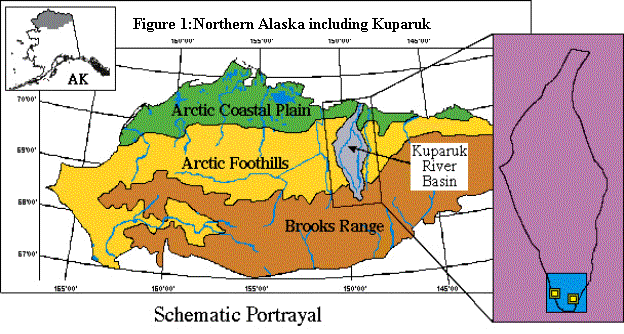
we will focus on the Kuparuk Basin, located in the North Slope of Alaska (shown
in Figure 1; Donald Walker,
http://www.Colorado.Edu/INSTAAR/TEAML/atlas/chapters/geobot.html). We will force the LSM with historical
climate data covering this basin and validate model-generated discharge, snow
extent, snow depth, and snow water equivalent across a range of spatial scales.
5 Modeling of the Land Surface
5.1 A Catchment Based Approach
To
put the proposed work in perspective, we present in this section the relevant
accomplishments of the ongoing NASA NSIPP project and emphasize how these
accomplishments can serve as the basis for new, valuable work.
Our
catchment-based land surface model (LSM) was developed to overcome a critical
deficiency in standard GCM-based LSMs, namely, the neglect of an explicit
treatment for spatial variability in soil moisture. Standard LSMs employ a one-dimensional treatment of subsurface
moisture transport and surface moisture and energy fluxes that effectively
assumes homogeneous soil moisture conditions across areas spanning hundreds of
kilometers. Much recent development
work by various groups has focused on improving the 1-D representation itself,
incorporating, for example, improved treatments of transpiration resistance and
even carbon budget models into the evaporation calculation. Relatively little attention has been given
to the spatial heterogeneity issue.
This is unfortunate given that this heterogeneity can have a strong,
even dominating, impact on surface energy and water budgets.
Our
strategy [Ducharne et al., 1998; Koster
et al., in review] calls for the partitioning of the land surface into a
mosaic of hydrologic catchments, delineated through analysis of surface elevation
data. When coupled to an atmosphere
model, the effective "grid" used for the land surface is not
specified by the overlying atmospheric grid.
Within each catchment, the variability of soil moisture is related to
characteristics of the topography and to three bulk soil moisture variables
through a TOPMODEL-type formulation of catchment processes. Care is taken, however, to ensure that the
deficiencies of the catchment model in regions of little to moderate topography
are minimized. Many of the ideas
underlying the strategy have been developed over a number of years by the Co-PI
Wood and his students [Famiglietti and Wood, 1991; Pauwels and Wood, 1999a; Peters-Lidard et al., 1997] and others [Bowling and Lettenmaier, in press; Nijssen et al., 1997; Stieglitz et al., 1997].
TOPMODEL
formulations permit for dynamically consistent calculations of both the partial
contributing area, and the baseflow which supports this area, from knowledge of
the mean depth of the water table and a probability density function (pdf) of
the soil moisture wetness index, c, derived from topography digital elevation
model (DEM) data. At any location, x,
within the watershed, the wetness index, c, defined to be ln(a/tanb)x, is the ratio
of the area, a, above any point on the catchment that drains
to the point x (a measure of how much water can potentially flow through this
location) to the local slope at that point, tan b, (a measure of the
potential driving water downslope through this location). As such, regions with a high topographic
wetness index, along valley bottoms and flatter areas, are regions of
convergent flow, a high water table, and in sum, constitute the bulk of the
saturated fraction of the watershed.
Regions with a low index, near the top of hills, are characterized by a
suppressed water table, and are primary recharge zones.
 A particularly unique aspect
of our catchment model is the separation of the catchment into three subareas,
each representing a distinct hydrological regime: one in which the surface is
saturated, one in which the surface is unsaturated but transpiration proceeds
without water stress, and one in which transpiration is stressed. Because these subareas are tied to the
dynamically varying moisture variables in the catchment, their sizes vary with
time. Key to the modeling strategy is the
application of different formulations of evaporation and runoff in each subarea
to reflect the fundamentally different physical mechanisms controlling these
fluxes in the three regions. This is a
far more physically consistent approach than is possible with traditional
one-dimensional LSMs.
A particularly unique aspect
of our catchment model is the separation of the catchment into three subareas,
each representing a distinct hydrological regime: one in which the surface is
saturated, one in which the surface is unsaturated but transpiration proceeds
without water stress, and one in which transpiration is stressed. Because these subareas are tied to the
dynamically varying moisture variables in the catchment, their sizes vary with
time. Key to the modeling strategy is the
application of different formulations of evaporation and runoff in each subarea
to reflect the fundamentally different physical mechanisms controlling these
fluxes in the three regions. This is a
far more physically consistent approach than is possible with traditional
one-dimensional LSMs.
The
catchment model has some additional components worthy of mention. A detailed snow model is now incorporated
into the code; this multi-layer model accounts for the coexistence of liquid
and solid phases, changes in snow density due to melting, refreezing,
compaction, density-dependent albedo, and other important processes [Lynch-Stieglitz,
1994; Stieglitz et al., in preparation]. Ground
thermodynamics are computed through a multi-level heat diffusion calculation. Transpiration and other surface energy
balance calculations proceed using established and tested code from a standard
``SVAT-type" vegetation model [Koster and Suarez, 1996; Koster and Suarez, 1992b] that includes bare soil evaporation and canopy
interception loss. The SVAT code used
for one-dimensional energy balance calculations is applied over each of the
three identified moisture regimes, and each regime maintains its own prognostic
temperature.
The
new catchment based model has been tested offline in two venues --- over the
Red-Arkansas basin, using forcing established for the PILPS 2c intercomparison
study [Wood et al., 1998], and over North America as a whole, using forcing
from the ISLSCP Initiative 1 CD-ROM [Sellers et al., 1996]. The
catchment boundaries and topographic-based model parameter values were derived
from the processing of GTOPO30 (1-km) DEM data; some 5000 catchments cover
North America, with 126 making up the Red-Arkansas basin.
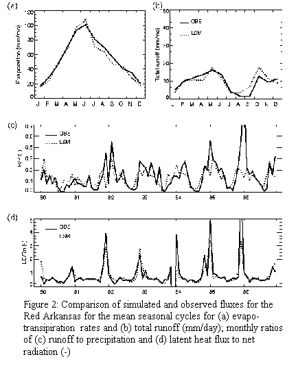
|
Figure 3: Model-predicted snow depth,
water equivalent snow depth, and snow pack
density for the 1970/71 snow season (solid line)
and observed snow characteristics at the NOAA-ARS
snow research station (stars). |
Results
for the Red-Arkansas are presented in Figure 2 [Ducharne et al., in review], which shows how model-simulated runoff and
evaporation compare with observed values.
(The evaporation ``observations" were derived from atmospheric
water budget calculations.) The
agreement between simulated results and observations is seen to be quite high,
especially given that the observations, while reliable, are associated with
some error. We must emphasize here that
the Red-Arkansas dataset was used in the development of the model itself, so
that some of the agreement seen in Figure 2 reflects a calibration of the model
physics. This calibration was
essentially limited, however, to the treatment of surface runoff generation
over unsaturated soil and cannot by itself explain the general agreement in
both the mean and variability of the simulated fluxes. Our main point here is that this model
framework is capable of reproducing observed evaporation and runoff rates over
large spatial scales. Note that because
different catchments below a single atmospheric grid cell exhibit different,
topography-dependent behavior, this modeling framework may be particularly
valuable for downscaling applications.
5.2 Snow and permafrost dynamics
While
sophisticated multi-layer snow models have been developed and successfully
applied at the local scale [Davis et al., 1995; Hardy et al., 1998; Jordan,
1995], the treatment of snow
processes, especially those used within GCMs, have been relatively simple. Some
models consider the winter snow pack only as a store of soil moisture [Abramopoulos
et al., 1988; Bonan, 1996; Koster and Suarez, 1996], while others blur the distinction between the snow
and the ground surface altogether by envisioning a composite soil and snow
layer [Dickinson et al., 1993; Pitman
et al., 1991]. Still others do distinguish between separate snow
and ground layers, yet represent the entire pack with a single snow layer regardless
of the actual pack depth [Slater et al., 1998]. However, most of these simple schemes have
considerable flaws. Lynch-Stieglitz [1994] demonstrated that an insufficient representation of
snow processes can lead to a corruption of surface energy fluxes and a
degradation of the snow insulation between the cold atmosphere and the warm
ground; ultimately impacting the seasonal development of ground freeze-thaw processes,
and compromising the normal hydrologic processes of runoff, ground water movement,
infiltration, etc., for a good part of the year. Further, Betts et al. [1998] have recently shown that an insufficient representation
of snow processes at high latitudes leads directly to a poor evolution of the
atmospheric boundary layer in weather forecasting models.
Recently,
sophisticated snow physics have been included in LSMs and demonstrate a clear
improvement in the overall simulation of the hydrologic cycle, including ground
freeze - thaw processes [Loth and Graf, 1998a; Loth and Graf, 1998b; Loth et al., 1993; Lynch-Stieglitz, 1994; Stieglitz
and Giblin, 1997; Stieglitz et al.,
1999b; Yang et al., 1997]. Typically, these multi-layer snow schemes explicitly
model the heat and mass (water) transport within the pack. Radiation conditions determine the surface
energy fluxes, and the heat flow within the pack is accomplished via linear
diffusion along the thermal gradient. Meltwater generated within a given layer
can drain to a lower layer, where it will refreeze, remain in the layer in the
liquid state, or pass through.
 As mentioned earlier, we
employ the snow model of Lynch Stieglitz et
al. [1994] coupled to the global catchment-based LSM of the NASA
NSIPP project. This three-layer snow model accounts for snow melting and
refreezing, dynamic changes in snow density, snow insulating properties, and
other physics relevant to the growth and ablation of the snowpack. As the boundaries of the snowpack move up
and down under the influence of snowfall, mechanical and wet compaction,
condensation, etc., three variables are needed to completely describe the
system; layer thickness (Zi),
water equivalent (Wi), and
heat content (Hi). The coupling to the catchment framework,
however, necessitated some modifications to the original scheme [Stieglitz
et al., in preparation]. In particular, we now ensure a smooth transition between
snow-free and snow-covered conditions in order to capture the gradual growth of
a snowpack's spatial extent and to avoid abrupt (discontinuous) changes in the
surface energy balance calculations.
The approach used is straightforward. We assume a minimum local snow
water equivalent, SWE, of 13 mm, a
value that allows the resolution of the diurnal surface temperature signal yet
still produces a stable solution with a 20-minute timestep. If a given volume of snow falls on a
snow-free catchment, that volume is spread uniformly over a fraction of the
catchment so that the local water equivalent at any snow-covered point is 13
mm. Thus, if the snow falling on a snow-free catchment during a timestep has a
total water equivalent volume, Vs,
and if the area of the catchment is A,
then the snow-covered areal fraction, As/A,
is taken to be V/(A*SWE).
The snow-covered areal fraction increases as more snow falls until As/A reaches 1, at which time
the local snow water equivalents across the catchment start increasing
uniformly. When the fractional coverage is less than one, the snow model is
represented with a single snow layer, whereas three model layers are used when
the snow coverage is complete [Lynch-Stieglitz, 1994]. The transition between the single layer and three
layer representations involves a simple conservative redistribution of layer
heat and water contents. Surface energy calculations are performed separately
over the snow free and snow covered areas.
As mentioned earlier, we
employ the snow model of Lynch Stieglitz et
al. [1994] coupled to the global catchment-based LSM of the NASA
NSIPP project. This three-layer snow model accounts for snow melting and
refreezing, dynamic changes in snow density, snow insulating properties, and
other physics relevant to the growth and ablation of the snowpack. As the boundaries of the snowpack move up
and down under the influence of snowfall, mechanical and wet compaction,
condensation, etc., three variables are needed to completely describe the
system; layer thickness (Zi),
water equivalent (Wi), and
heat content (Hi). The coupling to the catchment framework,
however, necessitated some modifications to the original scheme [Stieglitz
et al., in preparation]. In particular, we now ensure a smooth transition between
snow-free and snow-covered conditions in order to capture the gradual growth of
a snowpack's spatial extent and to avoid abrupt (discontinuous) changes in the
surface energy balance calculations.
The approach used is straightforward. We assume a minimum local snow
water equivalent, SWE, of 13 mm, a
value that allows the resolution of the diurnal surface temperature signal yet
still produces a stable solution with a 20-minute timestep. If a given volume of snow falls on a
snow-free catchment, that volume is spread uniformly over a fraction of the
catchment so that the local water equivalent at any snow-covered point is 13
mm. Thus, if the snow falling on a snow-free catchment during a timestep has a
total water equivalent volume, Vs,
and if the area of the catchment is A,
then the snow-covered areal fraction, As/A,
is taken to be V/(A*SWE).
The snow-covered areal fraction increases as more snow falls until As/A reaches 1, at which time
the local snow water equivalents across the catchment start increasing
uniformly. When the fractional coverage is less than one, the snow model is
represented with a single snow layer, whereas three model layers are used when
the snow coverage is complete [Lynch-Stieglitz, 1994]. The transition between the single layer and three
layer representations involves a simple conservative redistribution of layer
heat and water contents. Surface energy calculations are performed separately
over the snow free and snow covered areas.
To simulate ground freeze-thaw processes a
multi-layer ground schemes is used in which heat transport is physically modeled
via diffusion along the thermal gradient [Abramopoulos et al., 1988; Bonan, 1996; Stieglitz et al., 1997]. The scheme
has been tested for seasonal evolution of ground temperatures in regions
ranging from New England [Lynch-Stieglitz, 1994], to the Arctic [Stieglitz et al., 1999b], where permafrost dynamics plays a large role in the
seasonal hydrologic cycle.
Results at the Sleepers River watershed (8.4 km2),
located in the highlands of Vermont, demonstrate that all the features of snowpack
ripening that characterize pack growth/ablation are well simulated (Figure 3) [Lynch-Stieglitz,
1994].
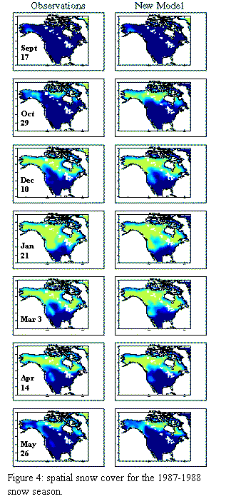
At
the Basin scale we can evaluate the ability of the coupled catchment-snow model
to simulate spatial coverage of snow, as well as snow amounts, over large
areas. To this end, ISLSCP data was used to drive the model over North America
for the period 1987 - 1988 and the Northern Hemisphere EASE-Grid Weekly Snow
Cover data set was used to evaluate simulated snow coverage. This successful larger-scale application of
the model at over the 5000 catchments comprising North America (Figure 4, [Stieglitz
et al., in preparation]) suggests that the global application of the model is
within reach, and more specifically, application to the arctic will be successful.
6 Detailed Work Plan
The
successful simulation of hydrologic and thermal processes using a land surface
model has several requirements. These requirements are:
1. A high quality model of the land surface processes for forecasting
of the LSM system states (ie. soil moisture, soil temperature, snow cover,
etc.).
2. Observations of the land surface forcing (meteorological data) for
driving the forecast of land surface system states when the LSM is running
off-line.
3. An appropriate spin-up strategy for initializing the LSM system
states.
4.
Remotely
sensed snow observation products, as well as ground observations, for
validating the LSM hindcast simulation of snow cover, snow depth and snow water
equivalent.
5.
River
discharge measurements, at a variety of scales for validating the LSM hindcast
simulation of catchement outflow, and flow routing.
We
will first outline our proposed approach and then detail the specifics in turn.
6.1 Proposed Approach
In
this approach the LSM is important for establishing the relationship between
snow, soil moisture, soil temperature, the energy and water budget. In order to
run the model (off-line from a general circulation model), high quality
meteorological data are required for forcing of the model. In addition to high
quality forcing data, the model forecast is dependent on the initial state
values given to the LSM. As the LSM states (other than snow which can be
observed via remote sensing), the LSM must be spun-up to realistic initial state
values prior to commencing the hindcast simulation. Hence, errors in the land
surface initialization, forcing data and LSM physics all contribute to some
errors in the forecast land surface states.
However, as the forcing data sets are long enough (30 - 40 years), this
problem should be mitigated as the run proceeds.
6.2 LSM Application to arctic regions
6.2.1
Snow Model Development
Here
we focus on those snow processes operating at the small catchment scale which
have a direct impact on our large Kuparuk basin scale simulations.
Stieglitz
et al (1999) has demonstrated that this TOPMODEL based modeling approach can be
used to successfully simulate the evolution of hydrologic and thermal processes
operating in the North Slope of Alaska.
Meteorological and hydrological data taken at Imnavait Creek from May
1991 through October 1993 (Hinzman and Kane) were used to force the land
surface model. Figure 5-7 shows monthly
averages of various watershsed water balance components for the period June
1991 through September 1993. With
freezing of the soil column beginning in early fall, soil moisture does not
change significantly until the onset of spring melt. As the pack ablates in late May and early June, melt waters
infiltrate the still frozen ground. The
soil is recharged and the mean water table depth rises from the previous summer
value nearly to the surface. The
associated partial contributing area increases from 20% to almost 40% (in good
agreement with McNamara et al. [1997]. Surface
runoff generated over the rapidly expanding saturated regions quickly enters
the stream system. As the soil active
layer deepens in the summer, evapotranspiration (and the latent heat flux)
begins to increase, peaks in July and August, and falls rapidly as the snow season
approaches. Finally, annual
precipitation is partitioned 47% into runoff and 53% into evapotranspiration;
the partitioning measured in the long-term field record. Modeled ground temperatures are in good
agreement with measurements.
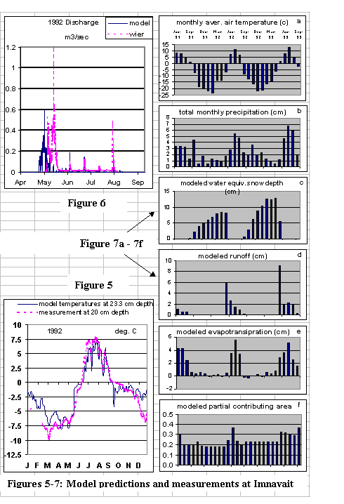 While the overall simulations
of discharge is adequate (Figure 4), even at these small spatial scales snow
heterogeneity significantly impacts the timing and quantity of snowmelt related
discharge and poses a obstacle towards application on an arctic wide
basis. Because the spatial distribution
of snow cover is not represented in the model framework, modeled snowmelt consistently
leads site data by five to ten days.
With high winds and low vegetation height, snow in this region of the
Arctic tends to blow into and accumulate in valleys [Kane et al., 1991; Liston, 1986; Liston and
Sturm, 1998]. As such, it
takes longer to melt a snowpack whose depth is substantially increased over a
reduced area compared to a pack that is uniformly distributed over the landscape. Further, as pointed out by Hinzman et al. [1996], where the snowpack is thick and dense on the valley
floor, it functions as a dam and holds back the water until the bonding
strength of the snow is overcome. As an
ongoing part of this effort we will improve the models representation of
sub-grid scale snow heterogeneity. To
account for the effects that wind, vegetation, and topography have on the distribution
of snow cover, we will adapt the work of Liston and Sturm [1998] to our modeling framework. While their spatially
explicit model is not directly compatible with the statistical treatment of
topography presented here, the empirical equations governing wind blown snow
can be used to treat snow distribution in much the same way we currently treat
soil moisture heterogeneity; through a statistical representation in which
valleys are regions of snow accumulation and uplands are regions of snow
ablation. Hartman et al. [1999] has recently applied such a procedure, albeit without
explicitly including for the effects of wind blown snow, and had success in improving
snowmelt discharge. In this respect
TOPMODEL formulations provide a clear advantage over more parameterized
hydrologic models such as VIC in that the TOPMODEL pdf does retain
quasi-explicit information about the landscape topography.
While the overall simulations
of discharge is adequate (Figure 4), even at these small spatial scales snow
heterogeneity significantly impacts the timing and quantity of snowmelt related
discharge and poses a obstacle towards application on an arctic wide
basis. Because the spatial distribution
of snow cover is not represented in the model framework, modeled snowmelt consistently
leads site data by five to ten days.
With high winds and low vegetation height, snow in this region of the
Arctic tends to blow into and accumulate in valleys [Kane et al., 1991; Liston, 1986; Liston and
Sturm, 1998]. As such, it
takes longer to melt a snowpack whose depth is substantially increased over a
reduced area compared to a pack that is uniformly distributed over the landscape. Further, as pointed out by Hinzman et al. [1996], where the snowpack is thick and dense on the valley
floor, it functions as a dam and holds back the water until the bonding
strength of the snow is overcome. As an
ongoing part of this effort we will improve the models representation of
sub-grid scale snow heterogeneity. To
account for the effects that wind, vegetation, and topography have on the distribution
of snow cover, we will adapt the work of Liston and Sturm [1998] to our modeling framework. While their spatially
explicit model is not directly compatible with the statistical treatment of
topography presented here, the empirical equations governing wind blown snow
can be used to treat snow distribution in much the same way we currently treat
soil moisture heterogeneity; through a statistical representation in which
valleys are regions of snow accumulation and uplands are regions of snow
ablation. Hartman et al. [1999] has recently applied such a procedure, albeit without
explicitly including for the effects of wind blown snow, and had success in improving
snowmelt discharge. In this respect
TOPMODEL formulations provide a clear advantage over more parameterized
hydrologic models such as VIC in that the TOPMODEL pdf does retain
quasi-explicit information about the landscape topography.
![]() Finally, we may find that
gradients in elevation are having an impact on snow heterogeneity. If so, a temperature lapse rate will be used
along with binned elevation bands to distribute snow cover and snow melt
throughout the landscape [Bowling and Lettenmaier, 1998; Hartman et al., 1999].
Finally, we may find that
gradients in elevation are having an impact on snow heterogeneity. If so, a temperature lapse rate will be used
along with binned elevation bands to distribute snow cover and snow melt
throughout the landscape [Bowling and Lettenmaier, 1998; Hartman et al., 1999].
6.2.2
Catchment Delineation
 Prior to any water and energy
balance simulations, two steps of data preprocessing must be performed;
catchment delineation and the calculation of the pdf of the TOPMODEL wetness
index, c, for each catchment.
Prior to any water and energy
balance simulations, two steps of data preprocessing must be performed;
catchment delineation and the calculation of the pdf of the TOPMODEL wetness
index, c, for each catchment.
The
NSIPP-LSM project currently uses the 1km resolution GTOPO30/HYDRO1k data to
calculate catchement wetness indices.
However, as demonstrated during the course of the NSIPP work and by
others [Wolock, 1998], 1km resolution data is insufficient to capture
hillslope processes. Systematic
recalibration of topographic index pdfs are therefore required for the reliable
estimation of TOPMODEL parameters.
However, throughout the North Slope of Alaska, high resolution, 60-90m
DEM data is available. Further, 10 m
data is available for a region of approximately 1000 km2 in the
Upper Kuparuk. For this study, this
high-resolution data will be used for catchment delineation and the estimation
of TOPMODEL parameters, obviating the need for recalibration.
The
study region will be segmented into a mosaic of indexed sub-catchments using a
delineation algorithm that includes a DEM error correction scheme. Each watershed index will permit access to a
pdf of c, a link into the drainage network template which permits river
routing, and a sub-catchment boundary geometry which facilitates meshing with a
GCM grid. The segmentation of
sub-catchments will be performed in tandem with estimation of hillslope and
channel network flow patterns using a multiple flow routing algorithm [Quinn
et al., 1991]. This
methodology permits robust estimation of the topographic index in addition to establishing
channel network structure and the along-channel properties required by routing
equations.
The
DEM flow routing algorithm is tied to an adaptive error correction (pit infill)
scheme, something that is particularly necessary during delineation of flow on
low relief areas such as coastal plains.
Generally, error correction schemes perform crude “flooding” operations
to force flow networks to join up, and to prevent internal drainage. In more difficult areas such as alluvial
plains, the artifacts that arise from this approach can cause non-negligible
errors in the estimated routing times along main channels. Our algorithm is similar to that of [Martz
and Garbrecht, 1998]: a quasi-diffusive, stochastic interpolation is performed
over pseudo-flat regions such that the interpolated flow routing is at least
roughly consistent with the topography around the area of error. This technique has been shown to be
successful for the delineation of braided flow patterns on error-prone DEMs of
alluvial fans, and will provide a solid basis upon which to build a regional
drainage model.
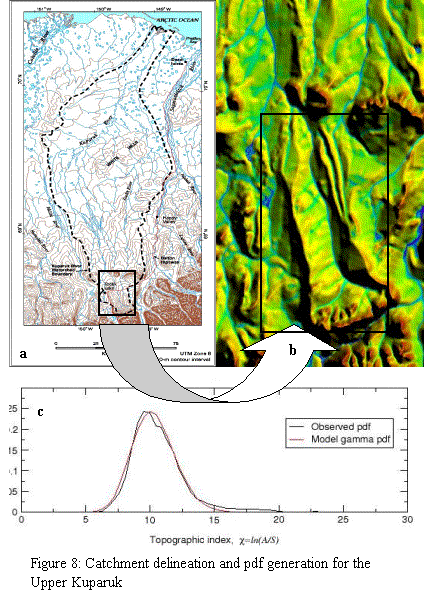
An
application of the use of smoothed 90m resolution data, and of the algorithms
for DEM correction and topographic index estimation, is shown in Figure 8 Figure 8a shows the Kuparuk drainage basin
(Donald Walker, www.Colorado.Edu/INSTAAR/TEAML/atlas/chapters
/geobot.html). Figure 8b shows a small
area of the Upper Kuparuk, about 32km by 50km in size, which contains the
Toolik Lake watershed in the center of the image. The colors in Figure 8b indicate the topographic index estimated
from the DEM; low values of c are shown in red (upslope regions), through green, to high values in
blue (valley regions). The pdf of c for the Upper Kuparuk River,
which includes Toolik Lake, are plotted in Figure 8c. Both the color image and the pdf show that the DEM error, which
is a potential problem in low relief areas to the north of Toolik Lake, and
also along the river valleys, is largely suppressed, and that robust estimates
of topographic index distributions can be obtained.
6.2.3
River routing
At each modeled timestep,
and for each sub-catchment, runoff is generated; surface runoff plus baselow. This runoff is then routed thorugh a DEM-based channel network to
provide model-estimated discharge at gauged discharge points within the
basin. The inclusion of the river routing
model, developed by Lohmann et al. [1998b] permits comparisons between the model-derived
discharge and observations at gaging stations.
This routing approach has been widely used with success in combining
land surface models to catchments and their gauged discharges [Lohmann
et al., 1998c; Maurer et al., in
review].
6.3 Land Surface Model Forcing Data
An
evaluation of the model will be undertaken over catchments in the Kuparuk
basin. High quality historical climate
data, available from 1960 through the present, will be used to force each of
the sub-catchments within the Kuparuk Basin. Measurements of river discharge,
snow extent, and snow depth, will be used to evaluate model performance. Test
catchments across a range of spatial scales will be employed; across length
scales where the channel routing transit time ranges from large to small
compared to the time scale of observation.
At the largest of scales we will evaluate model performance with respect
to simulating discharge into the Arctic Ocean via the Kuparuk river.
6.3.1
Model-generated
forcing data
The
use of high quality global atmospheric forcing of the land surface is essential
to produce reasonable land surface predictions. The off-line LSM requires wind
speed, air temperature, humidity, precipitation, and radiation on a sub-hourly
basis. Many of these forcing variables can be reliably provided by operational
Numerical Weather Prediction (NWP) models at NCEP, ECMWF, or NASA-DAO, run in
either a real-time or reanalysis mode. However, NWP models generally poorly
predict precipitation and radiation because the complex prediction of cloud
physics and dynamics, which can lead to gross errors in land surface
simulations, have not been mastered. Therefore, when available, we will use
observational products. Unfortunately
most high-quality long-term global land surface observations have been
processed on monthly time scales for use in climate variability studies, and
therefore lack the high temporal resolution required by land surface modeling
efforts. These low temporal resolution observations can still be used to
improve land surface predictions by reducing the longer- term land surface
forcing biases through a ratio correction. Essentially, NSIPP uses the NWP
model forcing as high-resolution temporal weights on the longer-term
observation averages when high-resolution observed forcing are
unavailable. [Pauwels, 1999] and [Pauwels and Wood, in review] have investigated the effect of substituting ECMWF
model data for observations over the BOREAS SSA and NSA. In their study, they found that the largest
errors in the forcing data is spring-time radiation due to the well-discussed
snow albedo bias problem [Betts and Ball, 1997] and precipitation, which is underestimated by about
40%. Betts and Viterbo [2000] have studied the water and energy balance from the
ECMWF model products for seven sub-basins of the Mackenzie River basin. Their analysis will provide an additional
basis for evaluating the use of NWP re-analysis products to force our LSM.
Generally
land-surface precipitation and radiation forcing is most critical to land
surface prediction, with surface winds, humidity, and air temperature being of
second-order importance. Therefore, using precipitation observations based on
gauges, GOES Precipitation Index (GPI) estimates [Arkin and Meisner,
1987], shortwave passive microwave (as available with the
SSM/I instrument, TRMM, and AMSR) estimates, and ground-based Doppler radar
estimates are a priority. The Global Precipitation Climatology Project (GPCP) [McCollum
et al., in review] has developed a long-term, globally continuous
combination of microwave, infrared, and gauge measurements that is an
attractive product for use in land surface modeling applications. Global
downward shortwave radiation fluxes are available [Pinker and Laszlo,
1992] using surface solar irradiance models. This is a
theoretical-spectral model and has shown success in producing the global
surface solar radiation flux using ISCCP C1 data as input [Whitlock
et al., 1993], and has been extended to use ISCCP D1 data. [Gupta,
1989] developed a parameterization for longwave surface
radiation using satellite measurements. Recently, he improved and modified the
algorithm [Gupta et al., 1992] for direct use of ISCCP D1 data. The use of air
temperature, winds, and humidity surface observations are also being explored
to improve land-surface predictions.
6.3.2
Observed forcing
data
Monthly data: Under the auspices of the
NSF project “Contemporary Water and Constituent Balances for the Pan-Arctic
Drainage system: Continent to Coastal Ocean Fluxes", a Pan-Arctic 0.25
degree gridded monthly data seta of precipitation and temperature for the
Pan-Arctic is now available for the period 1960 - 1990 (refs,
http://climate.geog.udel.edu/~climate/html_pages/archive2.html). In total, 8818 independent weather stations
north of 43N were used to produce the precipitation archive and 6487 stations
for the temperature archive.
Daily data: Global Summary of the Day
(GLOBALSOD) data contains precipitation, temperature, dew point, wind speed,
sea level pressure, and daily total sunshine.
Station coverage between latitudes 45N and 66N is extensive. Coverage above 66N is approximately 450
stations with nearly 100 stations in Alaska.
Hourly data: Alaskan surface weather
observations from 1901 through 1990 at approximately 150 stations are available
from the National Climatic Data Center (NCDC - DATSAV2 SURFACE). Data include precipitation, air temperature,
dew point temperature, wind speed, precipitation, station pressure, and cloud
cover. More specifically, since 1992
over a dozen meteorological stations have been set up throughout the Kuparuk,
all recording the requisite data needed to run the LSM
(ftp://arcss.colorado.edu/pub/projects2/climate/Alaska_NSlope_Met_1985-96/). With funding from ATLAS meterological stations
have now been established at Ivotuk, Alaska.
Finally, for all their deficiencies, two Wyoming snow gauges are located
with the Kuparuk basin, one at Imnavait Creek and one near Prudoe bay.
6.4 Land Surface Model Spin-up
Initialization
values for the system states of the LSM will be obtained by undertaking a land
surface spin-up. This will involve running the catchment-based LSM repeatedly
for a given year of forcing data, until the system states for the start of the
year converge to consistent set of values. The spin-up will be undertaken for
the first ten years of forcing data (i.e. 1960-1970). This will allow for
validation of forecasted system states from 1970 through to the present.
6.5 Validation Products
An
effective evaluation of any large scale modeling endeavor is always the most
difficult and yet most important aspect of the project. In this project, we
propose to evaluate the simulation using remotely sensed and ground observed
snow products of the snow cover, snow depth, and snow water equivalent, as well
as river observed discharge measurements throughout the Kuparuk basin.
6.5.1
Snow Observation
Products
Since
November 1978, the Scanning Multichannel Microwave Radiometer (SMMR) instrument
on the Nimbus-7 satellite, and the Special Sensor Microwave Imager (SSM/I) on
the DMSP series of satellites have been acquiring passive microwave data that
can be used to estimate snow extent and snow water equivalent. The SMMR
instrument failed in 1987, the year the first SSM/I sensor was placed in orbit.
On SMMR, the channels most useful for snow observations are the 18 and 37 GHz
channels. For the SSM/I, the frequencies are slightly different (19 and 37
GHz). Additionally, an 85 GHz channel is available on the SSM/I. This frequency
has been demonstrated to be beneficial in detecting shallow snow packs (< 5
cm thick). Passive microwave data for most places on the globe are available
for alternate days. The data are placed into ½ degree latitude by ½ degree
longitude grid cells, uniformly subdividing a polar stereographic map according
to the geographic coordinates of the center of the field of view of the
radiometers. Overlapping data in a cell from separate orbits are averaged to
give a single brightness temperature, assumed to be located at the center of
the cell. Because when the snow pack is wet, snow water equivalent information
is difficult to extract using passive microwave radiometry, only dry snow
conditions will be examined. This necessitates using only the nighttime
satellite overpasses so that there will be a higher probability that the snow
pack is not actively melting.
Remotely
sensed snow cover extent and snow water equivalent observations for all of the
Kuparuk will be produced from the twenty plus years of microwave brightness
temperature data. In addition to the passive microwave snow products, high
resolution (1 km or less) visible and near-infrared satellite data from
Landsat, the NOAA series of satellites and the DMSP optical sensors will be
employed to look at snow cover extent in more detail where warranted. Moreover, airborne gamma data are available
over much of the northern U.S. and southern Canada for the period from the late
1970s through the present time. This data set can be used to “spot check” the
passive microwave snow water equivalent products.
The
Northern Hemisphere EASE-Grid Weekly Snow Cover Extent data yields snow extent
data from 1971 through 1995. This
product is provided on a 25-km equal area grid and is available through NSIDC.
Daily
snow depth climatologies based on sit observations are available for 61 sites
throughout Alaska. The period 1949
through 1998 was used to construct the climatologies. The Data is available
from the Western Regional Climate Center.
Hourly/daily snow cover observations throughout Alaska from 1901 through 1990
at approximately 150 stations are available from the National Climatic Data
Center (NCDC). Finally, snow depth is
available from the GLOBALSOD data.
6.5.2
River discharge
products
Monthly data: Monthly Pan-Arctic
discharge data is now available from R-ArcticNet (http://www.R-arcticnet.sr.unh.edu/)
covering the period 1960 - 1990. In
total, this database encompasses 3700 gauged rivers. Unfortunately, this database does not include discharge
measurements within the Kuparuk basin.
We include the mention of this data with an eye toward eventual
Pan-Arctic application of the LSM
Daily data: The USGS currently
maintains about 88 full time stream-gauging stations in Alaska and about 40
"partial-record" stations used for peak flow data collection. Data
for some of these sites are available in real-time. Historical surface-water
data are available in a computerized database for about 2,600 sites. Daily
measurements for discharge within the Kuparuk Basin go back 20 years and exist
at three locations, the headwaters, the Kuparuk Crossing (where the Kuparuk
river and the Dalton Highway cross), and at Deadhorse Alaska (Prudoe Bay). At the smaller catchment scale is continuous
monitoring at the Toolik Lake inlet and at Imnavait Creek.
7 Simulations at ATLAS sites
In
addition to validating within the Kuparuk basin, and specifically, the Kuparuk
outflow into the Arctic Ocean, we will validate specifically at the ATLAS sites
where are large suite of data will be collected; including Barrow, Atquasuk,
Oumalik, and Ivotuk. Two sets of
experiments will be performed: (1) We will use the 1960-1990 historical climate
data mentioned above for regions near the ATLAS sites to force the LSM. The model will be validated against
site-specific measurements of ground temperatures, soil moistures, snow depths,
etc. Assuming a successful validation,
this experiment will be used to provide ecology models with a historical record
of sub-grid scale soil moisture and ground temperature against which they can
be tested and calibrated. (2) Forcing
the land surface model with the hydro-meteorological measurements currently
being taken under the auspices of the ATLAS program, we will be able to validate
model performance with a broad range of measurements, including the spatial
distribution of soil moisture, ground temperature, snow cover, surface water
and energy fluxes, and discharge. This
will provide invaluable insights into improving model physics.
8 Relationship to other ATLAS projects
These and related results will be of broad interest across
a range of disciplines, especially within the NSF Arctic Transitions in the
Land-Atmosphere System (ATLAS) program and amongst other arctic
researchers. It is our hope that this
pilot study will develop into a core hydrologic component of the ATLAS program and serve the needs of
ongoing ATLAS efforts. For example: We
hope to eventually (1) expand the scope of this modeling effort to the entire
Pan-Arctic, (2) couple our LSM with Amanda Lynch's ARCSyM regional climate
model with the aim of improving seasonal and inter-annual variability in climate
simulations, (3) use the model-generated sub-grid scale soil moistures and soil
temperatures to force ecology models such as GEM [Rastetter et al., 1991], TEM [Raich et al., 1991], CENTURY [Parton et al., 1987] and SPA [Williams et al., 1996]. Finally,
only through a proper accounting of arctic hydrologic and thermal processes,
and the validation of those processes, will we be in a position to determine
how the Arctic will respond to the expected warming in the next century. We feel this work leads us in that direction.
8 Schedule
This
project will be three years in duration. Activity during the first eighteen
months will focus on the catchment delineation, and the generation of TOPMODEL
statistics using the 10 m and 90 m available in the arctic (the NSIPP project
currently uses the 1 km DEM for catchemnt delineation), implementation of the
river routing algorithm, the development and implementation of a new sub-grid
snow scheme, and the processing of hydro-meteorological data. The second eighteen months will focus on
simulation and validation at scales ranging from small catchments, including
site specific validations at the ATLAS sites, to the entire Kuparuk basin.