
Monash University
School of Mathematics Sciences
2015


TASK 3
(to be returned on Friday 5th June or as early as possible)
Analyse and calculate the power spectrum of a time series of 24 h of observations of velocity oscillations of a small area on the sun. The data you are going to analyse represents the line of sight velocity field as measured by the instrument HMI on SDO. Choose a very small area of the Sun with a size 2x2 pixels, which corresponds to an area of 1''x1'' of the sun. The spatial resolution of the HMI/SDO images is 0.6'' per pixel. Calculate the power spectrum of the time series and identify the dominant frequency. Use the rectangular_mask code which generates a mask for your datacube. You will extract only the signal in the region of interest of the Sun. An autocorrelation analysis will also help you to identify the dominant frequency/period of the signal.
1. student will become familiar with the HMI/SDO maps of velocity of the Sun (Dopplergrams, each pixels measures m/s of displacement of the surface of the Sun). These maps show the Line Of Sight (LOS) surface velocity.
2. student will use simple Fast Fourier transforms to convert the original data from the space (x,t) into the space (kx,frequency). Students will identify dominant oscillations in the data (eq., the 5 min oscillation period in the Sun)
3. student will demonstrate skills in using any computer software package (visualizing FITS files, plot graphs) to be able to do a scientific interpretation of images
http://www.solarmonitor.org/full_disk.php?date=20111011
http://www.helioviewer.org/
Extract a few images as jpeg , different wavelengths, get familiar with the helioviewer site. I am hoping you will choose a few good events using the helioviewer, save the images or you can ask for movies to be saved, bring them on Friday to the CAVE.
Q1: Helioviewer is good for what? Answer by detailing the images available (size, wavelength, opacity role, visualization techniques)
Download also one single frame : DOPP_X_T.fits.0220.fits Create in Linux, in your home directory, a new directory with, let's say, the name SDO
>mkdir SDO
>cd SDO
make sure that from now on, you will do all your analysis in the SDO directory.
Download also the archived software SOFTWARE.tar . Untar it:
tar -xvf SOFTWARE.tar
Download also the archived software 00readme.txt .Read the 00readme file (inside) to follow instructions on how to make the codes executable in Linux (just type "make" in the same folder), and how to check that they work. Note: If you really want to work in Windows, fine by me. But you will need to be able to make the software run, read your datacube into the software, identify a mask and cropp a time series out of the cube, and fast fourier analysing.
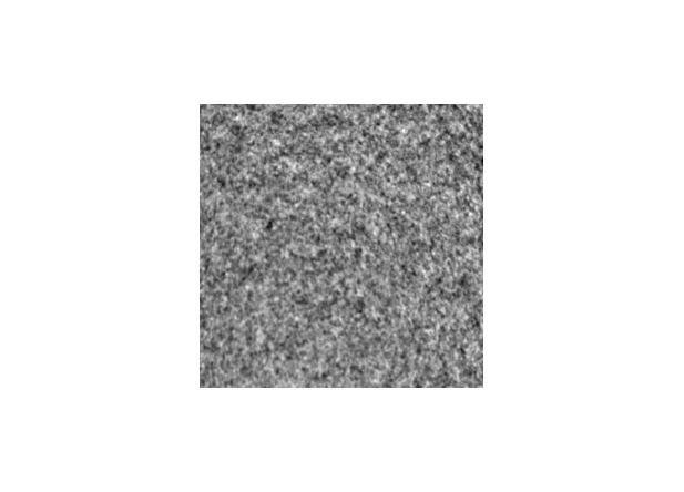
The datacube shows a sunspot (each stacked frame has sizes 256x256 pixels and represents 45 second of observation of the HMI LOS velocity of the quiet sun and a sunspot on the day 2011 October 11, around 17:00 TAI.
To get an idea about what has been cropped into your datacube:
A full-disk Dopplergram obtained at 06:00:00 UT on July 9, 1996 is shown below. The green rectangle shows the area of the Sun similar to the one cropped in DOPP_X_T.fits cube.
The white light image of the sun for the same day is also shown:
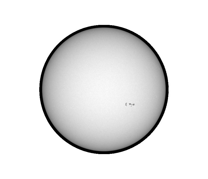
One single frame, in the datacube, has the field-of-view of 153 arcsec square, with a spatial resolution of 0.6'' :
Your datacube is a new one (data taken in 2011). You can analyse/visualize the cube using ds9 an executable file. The software ds9 is a very popular SAO display program.
You can see the cube in ds9 by typing:
ds9 DOPP_X_T.fits
You can see the 200th frame of the cube in ds9 by typing:
ds9 DOPP_X_T.fits.0220.fits
Q3: Look into the
header of the datacube (with ds9). What is the size
of a single FRAME: NAXIS1 =?, NAXIS2=?(number of pixels); DAXIS3 (units of sec)? How many frames have
been stacked together in this datacube? How many hours of
observations do correspond to the number of frames?
For your convenience, the frames have been already processed by removing the rotation of the Sun, and cropping around a sunspot that I analysed in the past. The original images were also Postel projected onto the frames that you see.
In order to read information from the Dopplergram from a particular region, we create masks. We are going to analyze the velocity oscillations of the Sun inside that particular MASK.
You should create a simple rectangular mask of 2x2 pixel size:
Usage: blank_frame NAXIS1 NAXIS2 frame_value output_filename >./blank_frame XX XX YY BLANK.fits
Example: rectangular_mask BLANK 50 50 52 52 MASK.fits
The rectangular_mask should avoid areas inside the sunspot. For comparison, you can choose later, a different mask inside the spot and compare the line of sight sunspot-velocity time series with those of the quiet sun values, to see how amazingly the magnetic field absorbs lots of the acoustic power of the oscillations in spots.
Then, you can visualize the MASK.fits (which is a FITS file) with ds9. Check that your mask is located where you wanted. It should look like this:
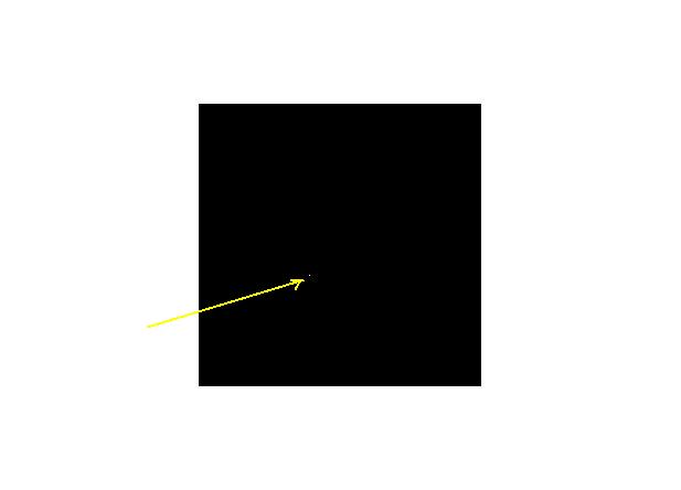

The white little spot has actually the size of 2x2 pixels. This is your mask!!!Very small!
Q4: What is the pixel
values of your mask? Why?
list_z_profile DOPP_X_T.fits MASK.fits > V.dat
Usage: list_z_profile filename [mask]
If you do not add "sign V.dat", the results will be displayed in your terminal. Using direction into V.dat means you pour the data into a data file V.dat (or whatever name). The list_z code calculates the averaged value of the surface velocity over an area defined by your own mask (first column is the number of frame - which is your time info; second column is the average value of velocity in the mask; second column is the root mean square value of velocity).Have a look at an image that shows the average of velocities in the cropped sun over 24 h. MEAN_IMAGE.fits Read the mean velocity values from the area defined by your mask and over plot this mean value as an horizontal line (Mean vs time) in your time series graph. Is the mean value of velocity where you expected?
So, the output is sent into a file V.dat which has three columns:
-first column: the time in number of frames. There is a time difference of 45 s between each frame.
-second column: the mean value of the pixels of the mask for each FRAME. These two columns will be your time series of the line of sight velocity (in km/s) versus time.
You should be able from now on to analyse the time series and produce a power spectrum. Read the data into an array and use a fast fourier transform to generate a power spectrum.
read_ascii3,file,x,y,z; oplot , x,y; NH=n_elements(y); NH2=floor(NH/2.); print,'NH=',NH; ;fourier transform of the signal; c=fft(y,-1); ;check the graph:; plot,abs(c),title='fft abs(c)' ,xtitle='k',ytitle='velocity (m/s)'; ;frequency resolution; delta_omega=2*3.1415/(NH*45.); delta_nu=delta_omega/(2*3.1415); frequencies=findgen(NH2)*delta_nu; times=1./frequencies; print,times(93); plot,times,abs(c),xrange=[0,1000],xtitle='time (min)',ytitle='velocity (m/s)';
Do not forget to write down in your report, what are the coordinates of the MASK you have chosen. Also watch for the conversion of frequecies back in units of time, as on the final graph you should show the time in minutes
Q5: Plot the time series of the LOS surface velocity (signal saved in file V.dat) and describe what you see (the visible periodicities, the amplitude of the signal, the length of the time series).
Using the Fourier transform function in IDL, or in Mathematica, or Matlab, calculate the power spectrum of the time series of file V.dat
Make your own research on how the fft function works in IDL or Mathematica or Matlab:
IDL>fft(data,-1)
Represent on a graph the power spectrum and describe its content. Do not forget the labels.
Q6:What frequency dominates the spectrum? What is the frequency resolution of the spectrum?
IDL>lag=dindgen(60)
IDL>print,lag
IDL>res=a_correlate(data,lag,/covariance)
IDL>plot,res,xtitle='min',ytitle='autocovariance'
Q8: What can you tell about the behaviour of the autocorrelation ? Can you identify in the autocorrelation plot the 5-min oscillation?